Discontinuity Analysis for Video
Processing
A dissertation submitted to the University of Dublin for the degree of Doctor of Philosophy
Hugh Denman
Trinity College Dublin, July 2007
iii
Abstract
This thesis is concerned with analysis of digital video through discontinuity detection. A discontinuity here is a sudden change that corresponds to some meaningful event in the video content.
The paradigm of discontinuity-based analysis is applied within three distinct contexts. Firstly, the problem of shot-change detection is explored. This amounts to the detection of signal-level discontinuities. An extensive review and bibliography of existing methods proposed for shot change detection are presented.
The next area of activity focuses on discontinuities as events, specifically in snooker video. It is described how many of the significant events within televised snooker play can be detected by targeted discontinuity detection, exploiting the characteristics of sports footage. Techniques for detecting ball pots and near misses, for summarising the episodes of play, and for tracking individual balls are described.
Declaration
I hereby declare that this thesis has not been submitted as an exercise for a degree at this or any other University and that it is entirely my own work.
I agree that the Library may lend or copy this thesis upon request.
Signed,
Hugh Denman
Acknowledgments
After a long period of immersive study, I think it fair to claim that I am at present the leading expert on the enduringly collegiate atmosphere of the Sigmedia group; my considered pronouncement is that you couldn’t hope to work with a better bunch of people. I particularly want to thank Dr Fran¸cois Piti´e, Dr Francis Kelly, and Andrew Crawford for the pleasure of working with them; Dr Claire Catherine Gallagher and Dr Naomi Harte for their invaluable help in preserving my sanity in the final days; and Deirde O’Regan, Dan Ring, and Daire Lennon for the enlivened atmosphere that attends them everywhere.
I have been generously funded in my research career by the Enterprise Ireland projects MUSE-DTV (Machine Understanding of Sports Events for Digital Television) and DysVideo, and the European Commission Framework projects BRAVA (BRoadcast Archives through Video Analysis) and PrestoSpace (PREServation TechnOlogy: Standardised Practices for Audiovisual Contents in Europe). The recent funding offered to the group by Adobe Systems Incorporated has provided for equipment that proved instrumental to the completion of the work described here. My thanks to all of these bodies.
Contents
Contents xi
List of Acronyms xvii
1 Introduction 1
1.1 Thesis outline . . . 2
1.2 Contributions of this thesis . . . 3
1.3 Publications . . . 4
2 Image Sequence Modelling 7 2.1 Image Sequence Modelling Overview . . . 7
2.1.1 Image-centric sequence modelling . . . 8
2.1.2 Scene-centric sequence modelling . . . 9
2.1.3 Affective sequence modelling . . . 9
2.2 Global Motion . . . 10
2.2.1 Global motion models . . . 10
2.2.2 Global motion estimation . . . 11
2.2.3 Robust estimation approaches . . . 11
2.2.4 Wiener solution approach . . . 13
2.2.5 Fourier domain approaches . . . 13
2.2.6 Integral projections . . . 14
2.3 Refined Global Motion Estimation for Simple Scenes . . . 14
2.3.1 Diagnosing GME Failure . . . 15
2.3.2 Recovering from GME failure . . . 16
2.3.3 Results and Assessment . . . 16
2.4 Local Motion Estimation . . . 18
2.4.1 Problem statement . . . 18
2.4.2 Correspondence matching . . . 19
2.4.3 Gradient-based methods . . . 20
2.4.4 Transform domain methods . . . 22
2.4.5 Bayesian methods . . . 22
2.5 Video Segmentation . . . 23
2.5.1 Motion segmentation . . . 23
2.5.2 Segmentation using motion and colour . . . 27
2.5.3 Video volume analysis . . . 27
2.5.4 Other approaches . . . 28
2.6 Multiresolution Schemes . . . 28
3 Video Shot Change Detection: A Review 29 3.1 Transitions in Video . . . 29
3.2 Shot Change Detection Systems . . . 32
3.3 Factors Complicating Shot Change Detection . . . 32
3.3.1 Similarity characteristics . . . 32
3.3.2 Film degradation . . . 34
3.3.3 Shot dynamics . . . 34
3.3.4 Editing style . . . 34
3.3.5 Non-Sequential Shot Structure . . . 35
3.4 Features for Shot Change Detection . . . 35
3.4.1 Direct Image Comparison . . . 37
3.4.2 Statistical Image Comparison . . . 39
3.4.3 Block Based Similarity . . . 42
3.4.4 Structural feature similarity . . . 45
3.4.5 Shot Modelling and Feature Clustering . . . 46
3.4.6 Frame Similarity in the Compressed Domain . . . 48
3.4.7 Genre Specific Approaches . . . 50
3.5 Transition Detection . . . 50
3.5.1 Thresholding . . . 51
3.5.2 Multiresolution Transition Detection . . . 53
3.6 Feature fusion . . . 53
3.7 Transition Classification . . . 54
3.7.1 Fade and Dissolve Transitions . . . 55
3.7.2 Wipe Transitions . . . 57
3.7.3 Transition classification from spatio-temporal images . . . 58
3.8 Statistical Hypothesis Testing . . . 58
3.9 Directions in Shot Change Detection . . . 60
4 New Approaches to Shot Change Detection 63 4.1 Cut Detection . . . 63
4.1.1 Frame Similarity Measure . . . 63
CONTENTS xiii
4.1.3 Peak Analysis in theδ Signal . . . 68
4.1.4 Mapping The Auxiliary Functions to a Probability . . . 70
4.1.5 Performance Evaluation . . . 72
4.2 Frame Similarity for Dissolve Detection . . . 72
4.2.1 Similarity Measure and Likelihood Distributions . . . 73
4.2.2 Peak Analysis in theδ22 Signal . . . 74
4.3 Model-Based Dissolve Estimation . . . 78
4.3.1 Dissolve model . . . 79
4.3.2 Global motion . . . 80
4.3.3 Local motion . . . 82
4.3.4 Examples ofα-curves . . . 83
4.3.5 Longer Dissolves . . . 83
4.3.6 Changepoints in theα-curve . . . 87
4.3.7 Dissolve Detection using theα-curve . . . 90
4.3.8 Comparison to other dissolve-detection metrics . . . 91
4.4 Integrated Dissolve Detection . . . 98
4.5 Conclusions and Future Work . . . 99
5 Detecting Snooker Events via Discontinuities 101 5.1 Related Work . . . 102
5.2 Preliminaries . . . 103
5.2.1 Shot-Change Detection . . . 104
5.2.2 Snooker Table Detection . . . 104
5.2.3 Table Geometry . . . 106
5.2.4 Player Masking . . . 108
5.2.5 Initial localisation . . . 110
5.3 Semantic Applications . . . 112
5.3.1 Clip Summaries . . . 112
5.3.2 Pot Detection . . . 114
5.3.3 Explicit motion extraction . . . 117
5.4 Conclusion . . . 120
6 Low-level Edit Point Identification 123 6.1 Instances of Percussive Motion . . . 124
6.1.1 Difficulties in Edit Point Localisation . . . 124
6.1.2 Assessment of Edit Point Detection . . . 125
6.2 Edit Point Identification using Amount of Local Motion . . . 127
6.2.1 Computing the Motion Trace . . . 128
6.2.3 Peaks in the Motion Trace . . . 132
6.2.4 Peak-relative location of edit points . . . 134
6.2.5 Peak Characteristics . . . 135
6.2.6 Peak Classification . . . 143
6.2.7 Edit Point Location and Peak Descent Slope . . . 146
6.2.8 Edit point detection using peak classification . . . 148
6.3 Edit Point Identification using the Foreground Bounding Box . . . 148
6.3.1 Filtering the bounding box traces . . . 150
6.3.2 Trace Extrema as Edit Points . . . 151
6.3.3 Mutual redundancy between bounding box traces . . . 152
6.3.4 Peaks in the bounding box traces . . . 152
6.3.5 Classifying bounding box trace peaks . . . 155
6.4 Motion Estimation Based Edit Point Identification . . . 157
6.4.1 Trace extrema as edit points . . . 159
6.4.2 Mutual redundancy between vector field traces . . . 159
6.4.3 Peaks in the vector field traces . . . 159
6.4.4 Classifying vector field trace peaks . . . 159
6.5 Motion Blur and Edit Point Identification . . . 163
6.5.1 Motion blur in interlaced footage . . . 163
6.5.2 Motion blur in non-interlaced footage . . . 165
6.5.3 Extrema detection in the motion blur traces . . . 165
6.5.4 Peaks in the motion blur traces . . . 167
6.5.5 Classifying motion blur peaks . . . 167
6.6 The Video Soundtrack and Edit Point Identification . . . 168
6.6.1 Maxima in the audio trace . . . 169
6.6.2 Peaks in the audio trace . . . 169
6.6.3 Peak classification in the audio trace . . . 169
6.7 Combined-Method Edit Point Identification . . . 169
6.7.1 Converting Traces to Edit Point Signals . . . 171
6.7.2 Combining Probability Traces . . . 176
6.7.3 Assessment . . . 182
6.8 Conclusion . . . 186
7 Segmentation For Edit Point Detection 191 7.1 Markovian Random Field Segmentation . . . 192
7.2 Colour Model . . . 193
7.2.1 Colourspace selection . . . 193
7.2.2 Distribution distance . . . 194
CONTENTS xv
7.3 The Edge Process . . . 195
7.4 Motion Models . . . 199
7.4.1 Cartesian / Polar vector representation . . . 199
7.4.2 Wrapping the vector angle distribution . . . 201
7.4.3 Vector models . . . 201
7.4.4 Vector likelihood . . . 203
7.5 Vector confidence . . . 203
7.5.1 Image Gradient Confidence . . . 203
7.5.2 Vector Confidence via the Mirror Constraint . . . 205
7.5.3 Vector Confidence via Vector Field Divergence . . . 205
7.5.4 Combining the Confidence Measures . . . 206
7.6 Encouraging Smoothness . . . 206
7.7 Label Assignment Confidence . . . 207
7.8 Changes in the Motion Content . . . 208
7.9 The Segmentation Process in Outline . . . 209
7.10 New Clusters and Refining the Segmentation . . . 211
7.10.1 The No-Match Label . . . 211
7.10.2 Splitting Existing Clusters . . . 212
7.10.3 Merging Clusters . . . 214
7.10.4 Cluster histories . . . 215
7.11 Segmentation Assessment and Analysis . . . 216
7.12 Conclusion . . . 220
8 Applications of Edit Point Detection 223 8.1 Interactive Keyframe Selection . . . 223
8.2 Motion Phrase Image . . . 224
8.2.1 MHI generation with global motion . . . 224
8.2.2 Finding the foreground map of a video frame . . . 229
8.2.3 Artificial rear-curtain effect . . . 229
8.3 Frame Synchronisation . . . 231
8.3.1 Related Work . . . 231
8.3.2 Beat detection . . . 233
8.3.3 Retiming the dance phrase . . . 233
8.3.4 Final points . . . 235
8.4 Conclusion . . . 236
9 Conclusion 237 9.1 Issues . . . 238
A Derivation of the optimal alpha value for dissolve modelling 241
B Sequence Sources 243
C Results 245
C.1 The Foreground Bounding Box . . . 245
C.1.1 Minima Detection . . . 245
C.1.2 Peak Classification . . . 249
C.2 Vector Field . . . 256
C.2.1 Minima Detection . . . 256
C.2.2 Peak Classification Distributions . . . 260
C.3 Sharpness . . . 268
C.3.1 Minima Detection . . . 268
C.3.2 Peak Classification . . . 269
C.4 Audio . . . 271
C.4.1 Maxima Detection . . . 271
C.4.2 Peak Classification . . . 272
List of Acronyms
DCT Discrete Cosine Transform
DFD Displaced Frame Difference
EM Expectation Maximisation
EMD Earth Mover’s Distance
GME Global Motion Estimation
HMM Hidden Markov Model
ICM Iterated Conditional Modes
IRLS Iteratively Reweighted Least Squares
LDA Linear Discriminant Analysis
LMM Local Motion Map
LMMSE Linear Minimum Mean Least Square Error
MAD Mean Absolute Difference
MAP Maximum a posteriori
MHI Motion History Image
MSE Mean Squared Error
ROC Receiver Operating Characteristic
SVD Singular Value Decomposition
1
Introduction
The digital video revolution began in earnest with the introduction of the DVD format in the mid-1990s. Since that time, vast quantities of digital video have been produced, through the increasing use of digital cinema technology in feature film production, the pervasive adoption of the DVD format for consumer video cameras, and the digitisation of film material for re-release in DVD and HD-DVD / Blu-Ray form.
Tools for manipulating digital video are thus in continuously increasing demand. A number of these software tools for video manipulation are available, and the capacity of these tools for digital video editing is increasing rapidly in line with the ever-expanding power of modern
computer systems. However, thenature of the operations which are facilitated by these systems
has remained essentially static, being limited to operations at the frame level. Manipulation using higher level concepts, such as shots, scene settings, and story arcs, is not available because
the content of the video is opaque within these systems. The development of content-aware
systems to address thissemantic gap is therefore an area of considerable research activity.
This thesis approaches content analysis through discontinuities. A discontinuity here is a
sudden change that corresponds to some meaningful event in the video content. This paradigm of discontinuity-based analysis is applied within three distinct contexts. Firstly, the problem of shot-change detection is explored. This amounts to the detection of signal-level discontinuities. The next area of activity focuses on discontinuities as events, specifically in snooker video. Here it is described how many of the significant events within televised snooker play can be detected by targeted discontinuity detection, exploiting the characteristics of sports footage. Thirdly, the detection of discontinuities in local motion is examined. It is shown that convincing analyses of
dance video can be created by exploiting these methods.
In each application area, the approach adopted is the extraction of a targeted description of the material, followed by the detection of discontinuities in this description. In shot change detection, the video is described in terms of frame-to-frame similarity; in snooker, the description targets the appearance of the table pocket areas and the ball tracks; and in dance video, the motion characteristics of the foreground region are extracted. In each case, discontinuities in the description of the media are found to correspond to time-points of interest in the video. This approach is applied successfully to feature extraction across a range of semantic levels: low-level in the case of shot changes, an intermediate level in the case of dance footage, and at a high semantic level in the case of snooker video.
1.1
Thesis outline
The remainder of this thesis is organised as follows.
Chapter 2: Image Sequence Modelling
This chapter describes the key ideas underpinning image sequence modelling, outlining the main approaches to global motion estimation, local motion estimation, and video segmentation. A new technique for detecting and recovering from global motion inaccuracies in ‘simple’ scenes is proposed. ‘Simple’ here refers to scenes with a well-contained foreground and a near-homogenous background; counter-intuitively, global motion estimation is particularly difficult in such video.
Chapter 3: Video Shot Change Detection: A Review
Here the problem of shot change detection in video is described and analysed in some depth. An extensive review and bibliography of the methods proposed for shot change detection are presented.
Chapter 4: New Approaches to Shot Change Detection
In this chapter, two new contributions to the problem of shot change detection are presented. The first is an approach to cut detection that performs well even in very difficult material. The second is a new dissolve detection scheme based on explicit modelling of the dissolve process. Both issues are considered as Bayesian classification problems.
Chapter 5: Detecting Snooker Events via Discontinuities
1.2. Contributions of this thesis 3
in terms of discontinuity detection. This chapter also introduces the use of Motion History Image (MHI) for summarisation of sports events, here snooker shots.
Chapter 6: Low-level Edit Point Detection
This chapter introduces the problem of edit point detection in dance video. An extensive analysis of various low-level approaches to edit point detection is presented, targeting several different descriptors of the motion content of the video. The chapter concludes with a probabilistic framework for fusion of these different descriptors for edit point detection.
Chapter 7: Segmentation For Edit Point Detection
In this chapter, a Bayesian video segmentation system is developed, designed for application to edit point detection in dance video. This application requires strong temporal coherence in the segmentation, particularly at motion discontinuities, and the novel contributions of this work are directed at these aspects.
Chapter 8: Applications of Edit Point Detection
Here three applications of edit point detection in dance video are described: interactive edit point browsing, dance phrase summarisation; and resynchronisation of dance video to new music.
Chapter 9: Conclusions
The final chapter assesses the contributions of this thesis and outlines some directions for future work.
1.2
Contributions of this thesis
The new work described in this thesis can be summarised by the following list:
A means for detecting and recovering from inaccuracies in global motion estimation in
simple scenes
Refinements to video cut detection particularly appropriate for very difficult sequences
A new technique for model-based dissolve transition detection
An algorithm for detecting full-table views in snooker footage
A perspective-invariant approach to recovering in-game geometry from snooker and tennis
An algorithm for detecting and masking out the player, where the player occludes the
table, in snooker
The use of the MHI for summarisation of sports events
A method for the detection of ‘ball pot’ and ‘near miss’ events in snooker based on
moni-toring of the pockets
A colour based particle filter approach to ball tracking, with applications to event detection
The use of motion detection, foreground bounding box analysis, vector field analysis,
motion blur analysis, and sound track analysis for the detection of edit points in dance video
Refinements to video segmentation incorporating the use of the Earth Mover’s Distance
(EMD) for colour modelling, polar co-ordinates for vector modelling, and motion histories for temporal coherence
The use of edit points in dance video for interactive keyframe selection and dance phrase
summarisation
The exploitation of edit points in dance video and music beat detection for real-time
resynchronisation of dance with arbitrary music
1.3
Publications
Portions of the work described in this thesis have appeared in the following publications:
“Content Based Analysis for Video from Snooker Broadcasts” by Hugh Denman, Niall
Rea, and Anil Kokaram, in Proceedings of the International Conference on Image and
Video Retrieval 2002 (CIVR ’02), Lecture Notes in Computer Science, vol. 2383, pages 186–193, London, July 2002.
“Content-based analysis for video from snooker broadcasts” by Hugh Denman, Niall Rea,
and Anil Kokaram, in Journal of Computer Vision and Image Understanding - Special
Issue on Video Retrieval and Summarization, volume 92, issues 2-3 (November - December 2003), pages 141-306.
“A Multiscale Approach to Shot Change Detection” by Hugh Denman and Anil Kokaram,
inProceedings of the Irish Machine Vision and Image Processing Conference (IMVIP ’04), pages 19–25, Dublin, September 2004.
“Gradient Based Dominant Motion Estimation with Integral Projections for Real Time
1.3. Publications 5
Anil Kokaram, inProceedings of the IEEE International Conference on Image Processing
(ICIP’04), volume V, pages 3371-3374, Singapore, October 2004.
“Exploiting temporal discontinuities for event detection and manipulation in video streams”
by Hugh Denman, Erika Doyle, Anil Kokaram, Daire Lennon, Rozenn Dahyot and Ray
Fuller, inMIR ’05: Proceedings of the 7th ACM SIGMM International Workshop on
Mul-timedia Information Retrieval, pages 183–192, New York, October 2005.
“Dancing to a Different Tune” by Hugh Denman and Anil Kokaram, in Proceedings of
2
Image Sequence Modelling
In this chapter the imaging process is introduced and an overview of image sequence modelling techniques is presented. A new technique for refining global motion estimation in sequences with low background detail is described. For additional material on the essential principles of digital image processing, the reader is referred to the excellent book by Tekalp [298].
2.1
Image Sequence Modelling Overview
Figure 2.1 illustrates the three essential stages in the video process. A camera or other imaging device is directed towards a three-dimensional scene in the real world, and captures a two-dimensional projection of this scene. These images are recorded in succession to some storage
Scene Imaging System Viewer
FrameStore
Figure 2.1: Stages in an imaging system
medium. Finally, the images are presented to a viewer through some display technology. To apply digital signal processing techniques to film, it is necessary that the film be available in digital format. Modern video and film cameras record directly to digital, typically through the use of a charge-coupled device, or CCD, as the light sensor. Early video cameras record by analogue means, such as onto magnetic tape or optical film. This film can subsequently be
digitised in a separate stage. In either case, the result is adigital image sequence.
A digital image sequence is an ordered set of N rectangular arrays {In(x) : 0≤ n < N}.
Herenis the temporal index of the image in a sequence, andx= (r, c)T denotes the pixel site at
rowrand columncof the image. For intensity images, In(x) is scalar valued; for colour images,
In(x) is a vector indicating intensity and colour—for example, a three-tuple representing red,
green, and blue light intensities at the site.
For an image sequence arising from the continuous operation of one camera, changes in pixel intensity are caused by four distinct processes. First, changes in the orientation and position of the camera change which portion of the scene is depicted; this is the camera motion process. To an observer, the scene background appears to move relative to the image space. As this
perceived motion is coherent across the entire image plane, it is termedglobal motion.
Secondly, individual objects in the field of view of the camera may themselves move; this is designated object motion, or local motion. This motion may be translational or rotational, and can include changes in size and self-occlusion.
Thirdly, changes in the illumination incident on the depicted scene will affect the readout values of the image acquisition device.
Lastly, flaws and aberrations in the acquisition device, the digitisation process, or arising during storage of the sequence, introduce noise to the image sequence.
An image sequence model is a set of hypotheses concerning the nature of the material de-picted. From these hypotheses, constraints can be derived. These constraints facilitate analysis of the variations at pixel sites over time in terms of the four processes identified above.
2.1.1 Image-centric sequence modelling
The essential hypothesis underlying image-centric sequence modelling is that the images depict objects that are much larger than the pixel size. Thus adjacent pixels with similar intensity values are likely to depict the same object.
Many image processing applications rely on constraints introduced by this hypothesis. Spa-tial noise reduction, for example, exploits the constraint that object surfaces should be smooth. Motion estimation generally relies on the constraint that adjacent pixels move identically, as described below.
2.1. Image Sequence Modelling Overview 9
for the effects of occlusion and revealing. The layer model proposed by Wang and Adelson [321] supercedes this rubber sheet model in these respects.
The directly perceived motion in a sequence is due to the displacement of spatial gradients. The motion of the gradients is termed optic flow. Motion that does not result in the displacement of gradients cannot readily be extracted from the sequence. For example, if a camera is directed at a rotating smooth sphere under constant illumination, no optic flow results [149]. Optic flow estimation is then the analysis of the motion through gradients.
2.1.2 Scene-centric sequence modelling
The hypotheses underlying scene-centric sequence modelling are in fact a description of the imaging process itself. In other words, scene-centric sequence modelling treats video explicitly as the perspective projection of three-dimensional objects onto the imaging plane. The goal is to recover as much information as possible about the configuration of the objects being projected, in terms of their relative position and size, the lighting conditions obtaining, and their three-dimensional motion. Optic flow estimation is an essential precursor to scene-centric modelling. The difficulty with this approach is that deriving constraints on the image sequence is very difficult with a scene-centric model. For example, Nagel in [231] illustrates the ambiguity be-tween changes in object depth (motion perpendicular to the image plane) and changes in object size. Further ambiguities arise from illumination effects: changes in the light source and shadows can result in intensity changes that are difficult to distinguish from motion. Even assuming that object size and illumination are constant, recovering the three-dimensional scene from the optic flow involves inherent ambiguities [3, 295, 338].
The scene-centric approach has been more common in the computer vision community than in signal processing, and has resulted in a very considerable body of research [110, 138].
2.1.3 Affective sequence modelling
Inasmuch as scene centric modelling considers real world objects rather than patches of pixels, it is a higher level approach than image-centric modelling. Essentially, scene-centric modelling en-compasses both the scene and imaging stages shown in figure 2.1, while image-centric modelling is only concerned with the imaging stage. The next level of video modelling, then, encompasses all three stages, including the human observer.
human observer, the scope and relevance of computer-assisted media processing will increase to encompass these affective aspects.
2.2
Global Motion
A marked distinction is drawn in the literature on motion estimation between global motion
estimation andlocal motion estimation[298]. In practical terms, this distinction is well founded. However, from a theoretical standpoint, one is always fundamentally concerned with an image equation of the form
In(x) =In−1(F(x, θ)) +(x) (2.1)
The vector functionF(x) represents co-ordinate transformation according to the motion model,
parameterized byθ. The term(x) represents errors arising from noise in the image sequence, or
due to model inadequacy. In this section, motion modelsF(x,Θ) suitable for global motion are
described, along with the means of estimating, or fitting, these models to the data. Section 2.4 section describes local motion models and estimation techniques.
2.2.1 Global motion models
Global motion estimation methods attempt to fit a single, low-order motion model to the image sequence contents as a whole. An accessible discussion of global motion models and their rep-resentational capacities has been presented by Mann and Picard [213]. The simplest choice for
the form of Fis the translational model, Θ= (dx, dy),F(x, θ) =x+ [dx, dy]T. The commonly
used affine model is given byΘ= (A,d),F(x, θ) =Ax+d. Here,A is a 2×2 transformation
matrix accounting for scaling, rotation, and shear; d = [dx, dy]T as before. This is the model
used throughout this thesis for global motion estimation. Higher-order models, including bilin-ear and biquadratic models, can also be applied. These models are linbilin-ear in that they can be written in the form
F(x,Θ) =B(x)Θ (2.2)
whereB(x) is a matrix-valued function ofx. For example, in the case of the affine model,
B(x) =
"
x1 x2 1 0 0 0
0 0 0 x1 x2 1
#
Θ = [a1, a2, d1, a3, a4, d2]T (2.3)
whereai,di, andxi are the components of A,d, and x.
The eight-parameter projective transform takes
F(x,Θ) = Ax+d
2.2. Global Motion 11
This model can exactly account for all changes due to camera motion, assuming that the scene contents are effectively planar (the zero-parallax assumption). However, this is a non-linear
transform1, and as such more difficult to solve.
2.2.2 Global motion estimation
Once a model for the global motion has been chosen, it is necessary to estimate the parameters that best account for the observed image data. Global motion estimation is normally carried
out between a pair of frames In, In−1. The error associated with some parameter values Θ0 is
assessed via the Displaced Frame Difference (DFD)
DFDΘ(x) =In(x)−In−1(F(x,Θ)) (2.5)
In general parameter estimation terminology, the DFD measures the residuals for parameters
Θ. The aim then is to find the optimal parameters ˆΘminimising some function of the DFD. A
least squares solution, for example, entails solving
ˆ
Θ= arg min
Θ
X
x
DFD2Θ(x) (2.6)
DFD(x) will have a high value if the parameters ˆΘ do not describe the motion at site x.
For inaccurate parameters, this will be over much of the image. However, at sites xcontaining
local motion, DFD(x) will take a high value for all parameter values. Thus the minimisation
technique adopted should be robust against outliers.
2.2.3 Robust estimation approaches
Odobez and Bouthemy [244] applied an M-estimation approach to robust estimation for global motion parameters. In M-estimation, the aim is to solve
ˆ
Θ= arg min
Θ
X
x
ρ(DFDΘ(x)) (2.7)
where rather than squaring the DFD, a function ρ(.) is used to limit the influence of large
residuals on the optimal parameters. This formulation is equivalent to solving
ˆ
Θ= arg min
Θ
X
x
w(x) DFD2Θ(x) (2.8)
for suitable weights at each site [351].
1In the sense thatx0
=F(x,Θ) is related toxby
" x0
1
x0
2
#
= "
x1 x2 1 0 0 0 −x1x01 −x2x01
0 0 0 x1 x2 1 −x1x02 −x2x02
#
·[a1, a2, d1, a3, a4, d2, c1, c2]T
withx0
The optimal parameters ˆΘare determined using an iterative scheme. Two factors motivate
the iterative approach. Firstly, a Taylor series expansion must be used to linearise DFD(x) with
respect toΘaround some initial estimate Θ0. Thus, for some updateu, the weighted DFD at
x, WDFDΘ0+u(x), is found by
WDFDΘ0+u(x) =w(x)In(x)−In−1(B(x)Θ0)− ∇In−1(B(x)Θ0)B(x)u+ ˆ(x) (2.9)
where ˆ(x) represents both the higher-order terms of the series and the error term. The Taylor
series expansion is only valid for small updatesu, and as such is applied iteratively until some
convergence criterion is met (typically a threshold on the magnitude of u). This also suggests
that a multi-resolution scheme be employed, as described in section 2.6.
The second reason that iterative estimation is used pertains to the choice of weights. The
weight at a sitexshould be high ifx is subject to global motion, and low otherwise. Thus, the
ideal weights can only be determined where the global motion is already known. The weights and parameters are therefore estimated iteratively, resulting in an Iteratively Reweighted Least Squares (IRLS) estimation scheme.
At each iteration i, the value ofu for which
∂WDFD(x)
∂u = 0 (2.10)
is found. This value is given by
ˆ
u= [GTWi−1G]−1GTWi−1z (2.11)
HereGis the matrix of gradient values{∇In−1(B(x)Θi−1)B(x)}x,Wi is the vector containing
the weights over the entire image, andz is the vector of residuals{Inx−In−1(B(x)Θi−1}x.
Given the parameters Θi at iterationi, the weightsWi can then be found by
w(x) = ρ(DFDΘi(x))
DFDΘi(x)
(2.12)
where various choices for ρ can be used [351]. In [244], Tukey’s biweight function [156] is used
forρ.
Dufaux and Konrad [93] also use M-estimation, with the function ρ taken as
ρ(e) =
(
e2 if|e|< t
0 otherwise (2.13)
The thresholdtis chosen at each iteration so as to exclude the top 10% of absolute DFD values.
2.2. Global Motion 13
2.2.4 Wiener solution approach
Kokaram and Delacourt presented a Wiener-based alternative for finding the parameter up-date [182]. In this approach,
ˆ
u= [GTWG+µwI]−1GTWz (2.14)
This introduces the regularising termµw = σ2ee/σuu2
, whereσ2eeis the variance of the residuals
and σ2
uu is the variance of the estimate for ˆu. In practice, µw = |Wz|λλ∧∨, where
λ∧
λ∨ is the
condition number of [GTWG+µwI]. This regularisation limits the update where the matrix is
ill-conditioned or where the DFD takes large values. Binary weights are used in [182], although other weighting functions could be used.
2.2.5 Fourier domain approaches
The normalised cross-correlation of two images can be efficiently computed in the spatial fre-quency domain using the Fast Fourier Transform (FFT). This suggests an efficient approach for
computing translational displacement between two images. LetInand In−1 be two frames that
differ only by a displacement d= [dx, dy] such that
In(x, y) =In−1(x+dx, y+dy) (2.15)
The corresponding Fourier transforms, Fn and Fn−1, are related by
Fn(u, v) =ej2π(udx+vdy)Fn−1(u, v) (2.16)
The cross correlation function between the two frames is defined as
cn,n−1(x, y) =In(x, y)~In−1(x, y) (2.17)
where~denotes 2-D convolution. Moving into the Fourier domain results in the complex-valued
cross-power spectrum expression
Cn,n−1(u, v) =Fn(u, v)Fn∗−1(u, v) (2.18)
where F∗ is the complex conjugate of F. Normalising Cn,n−1(u, v) by its magnitude gives the
phase of the cross-power spectrum:
˜
Cn,n−1(u, v) =
Fn(u, v)Fn∗−1(u, v)
|Fn(u, v)Fn∗−1(u, v)|
=e−j2π(udx+vdy)
(2.19)
Taking the inverse Fourier transform of ˜Cn,n−1(u, v) yields the phase-correlation function
˜
which consists of an impulse centered on the location [dx, dy], the required displacement.
The phase correlation method for translation motion, then, involves evaluating (2.19) and taking the inverse Fourier transform. This yields a phase correlation surface; the location of the maximum in this surface corresponds to the translational motion. Sub-pixel accuracy can be obtained with suitable interpolation.
Phase correlation for translational motion was presented by Kuglin and Hines in 1975 [186], for registration of astronomical images. In 1993, Bracewell published the affine theorem for the two-dimensional Fourier transform [44]; a number of researchers then developed Fourier-domain systems for affine image registration [209, 261] and global motion estimation [147, 188]. An accessible presentation of how Fourier domain methods can be used for affine global motion estimation appears in [167, appendix A].
2.2.6 Integral projections
The vertical and horizontal integral projections Inv,Inh of an imageIn are the vectors formed by
summing along the rows (respectively columns) of the image:
Inv = X
x
In(x, y) (2.21)
Inh = X
y
In(x, y) (2.22)
The use of integral projections was originally proposed by Lee and Park in 1987 for block matching in local motion estimation [191], described further below. In 1999, Milanfar showed that motion estimation applied to these two one dimensional vectors reveals the global motion of the image itself [222]. This work considered integral projections as a form of Radon transform, and established the theoretical soundness of the approach on this basis; the affine motion model is used. A differently motivated analysis appears in [71], targeting translation motion. The appeal of this approach lies in its simplicity of implementation and suitability for real-time applications.
2.3
Refined Global Motion Estimation for Simple Scenes
2.3. Refined Global Motion Estimation for Simple Scenes 15
(a) Video frame (b) Result of inaccurate GME (c) Result of accurate GME
Figure 2.2: Improvement in global motion estimation wrought by excluding the foreground region. The DFD after global motion compensation is superimposed in red in (b) and (c), along with its bounding box.
global motion model here is affine, with multiplicative parameter A and translation parameter
d.
2.3.1 Diagnosing GME Failure
As described above, the DFD at framenafter global motion estimation is the difference between
compensated frame n−1 and framen:
DFD(x)n =In(x)−In−1(Ax+d) (2.23)
Where GME has been successful, all the energy in the DFD will correspond to foreground regions of the image sequence. Figure 2.2 shows DFDs for successful and unsuccessful motion
estimation. Figure 2.2 (a) shows a frame from the greenDancer sequence. There is no camera
motion at this frame of the sequence. Image (b) shows the DFD energy and bounding box in red, after inaccurate global motion estimation. The DFD bounding box is the smallest rectangle containing all non-zero elements of the DFD image. Image (c) shows the DFD energy and bounding box after successful global motion estimation, using the technique described here. Where GME is accurate, the DFD bounding box corresponds to the foreground region of the frame.
Although the region of the frame corresponding to the foreground cannot be known in advance, it can be assumed that GME is accurate more often than not, and so the DFD bounding box usually contains the foreground motion. This assumption is generally justified, particularly at the start of a sequence as the subject begins to move. Any sudden change in the DFD bounding box can then be interpreted as an indication of GME failure.
The bounding box at frame nis defined by four components, for its top, bottom, left, and
right locations: BBn = [BBtn,BBbn,BBln,BBrn]. Given the bounding boxes of the previous
bounding box in the current frame. Hence BBtn ∼ N(BBt, σt2) and similarly for the other
bounding box components. These components can be estimated using thekmeasurements from
the previous frames by
BBt = 1 k
n−1 X
j=n−k
BBtj (2.24)
σt2 = 1 k
n−1 X
j=n−k
(BBtj−BBt)2 (2.25)
GME failure is then diagnosed if any component k lies outside the 99% confidence interval for
the associated Gaussian, i.e. where
BBk−BBk
>2.576σk (2.26)
2.3.2 Recovering from GME failure
Once GME failure has been diagnosed at a particular frame, various methods to improve the estimate can be employed. The simplest approach is to exploit the fact that camera motion is temporally smooth in most cases, by proposing the GME parameters from the previous frame
as candidate parameters for the frame causing difficulty. These are designated θ2. A second
candidate set of parameters can be generated by performing GME a second time, but excluding the region inside the DFD bounding box of the previous frame from the estimation. This prevents the foreground motion from affecting the global motion estimate. The resulting parameters are
designated θ3. A third, related candidate is generated by finding the median of the lastN = 25
DFD bounding boxes, designated the median foreground rectangle. GME is then performed
with this region excluded from estimation, and the parameters found are designatedθ4.
In cases where GME failure has been diagnosed, there are thus four candidate sets of parameters–the original parameters and the three alternatives described above. These are
des-ignated θi, with i ∈ {1. . .4}. Each of these parameter sets is used to generate a DFD, and
the bounding box of each DFD image is found. The set of GME parameters resulting in the DFD bounding box having the closest match to the historic distribution is selected as the best
estimate for the current frame. Specifically, the selected parameters for frame n, θn={A,d},
are found by
θn=θˆı, where ˆı= arg max
i∈{1...4}
X
k∈{t,b,l,r}
exp
(BBkni −BBk)2
σk
(2.27)
Here BBkni is bounding box component kresulting from candidate parameters θi.
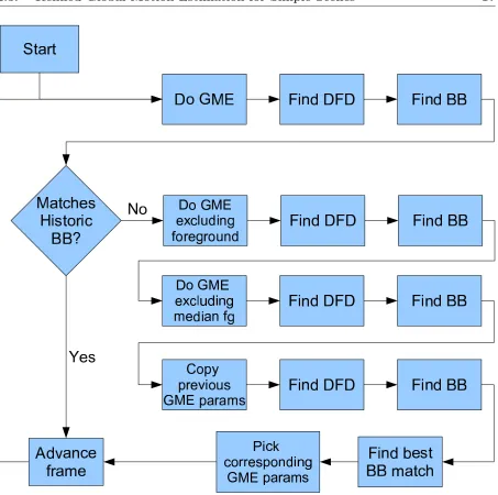
The procedure is illustrated in flowchart form in figure 2.3.
2.3.3 Results and Assessment
2.3. Refined Global Motion Estimation for Simple Scenes 17
Figure 2.3: The GME refinement algorithm. ‘BB’ stands for the DFD bounding box. The ‘BB match’ refers to the similarity between the current DFD bounding box and those found in previous frames.
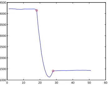
possible. Figure 2.4 (a) shows the location of the bottom edge of the DFD bounding box over 80
frames of thegreenDancer sequence, identified by unmodified GME and also using the technique
described here. The refinement technique results in a considerably smoother signal, indicating that GME performance has been improved.
Figure 2.4 (b) shows how often each set of global motion parameters was selected when
the refinement technique was applied to the 1900 frame greenDancer sequence. The initial
parameters, θ1, were found to be a poor match to the historic distribution in 699 cases. In
120 140 160 180 200 0
50 100 150 200 250 300
Frame
Row
Without Refinement With Refinement
(a) Location of DFD bounding box bottom edge using unrefined GME and the technique described here. The
plot covers 80 frames from thegreenDancer sequence.
0 100 200 300 400 500
n
θ1 θ3 θ2 θ4
(b) Selection counts of different candidate parameters. N=699.
Figure 2.4
that the refinement is being invoked somewhat more than necessary, and that a looser fit to the historic distribution should be considered a match. Of the three alternative candidate
parameters,θ3 most often results in the closest-matching bounding box, but each alternative is
selected for some frames.
Video material illustrating the application of this approach to a number of sequences is provided in the accompanying DVD. These videos demonstrate that the technique results in a considerable improvement in GME accuracy for numerous frames. It is noted that this technique should not be incorporated into GME systems by default, but rather selected by an operator for application to suitable sequences.
2.4
Local Motion Estimation
The problem of local motion estimation in image sequences has been the target of consider-able research effort over a number of decades. A brief overview of the principles and principal techniques is presented here. Comprehensive review material is available in a number of publi-cations [94, 214, 230, 288, 298, 314].
2.4.1 Problem statement
In local motion estimation, the aim is to describe the motion of each region of the image
2.4. Local Motion Estimation 19
model F(x,Θ) varies with the sitex. The most commonly used formulation is
F(x,Θ) =x+dn,n−1(x) (2.28)
Here dn,n−1(x) is a vector field describing the translational motion at each pixel. The effects of
zooming and rotation can be approximated as translational motion provided the motion between frames is small.
Numerous approaches to fitting a model of the form (2.28) to an image sequence have been developed, and will be outlined here. It is first noted that (2.28) fails to account for the effects of occlusion and revealing in the image sequence. These effects are found in all sequences containing motion: as any object moves, it will occlude some areas of the previous frame and reveal others. Modelling these effects requires extensions to the motion model that are not described here; approaches addressing this issue have been presented in [31, 160, 179, 184, 286].
Consider motion estimation in video having dimensionsM×N pixels. There are then M N
equations of the form
In(x) =In−1(x+dn,n−1(x)) (2.29)
and each equation is to be solved for the two components of d(x). There are thus twice as
many unknowns as there are equations, and so the problem is underconstrained. In fact, at
each site x, only the motion prependicular to the gradient atxcan be estimated, known as the
‘normal flow’ [298, pp. 81-92]. This difficulty is known as the aperture effect, because in effect the aperture, or window, used for motion estimation is too small.
The most common way of dealing with this difficulty is to assume that the motion is constant
over some window larger than one pixel, typically a blockB pixels on a side. Motion estimation
within the block is then described byB2equations with two unknowns in total, and the problem
is no longer underconstrained. Motion estimation over blocks of pixels also improves resilience to noise in the image sequence. The aperture effect can still arise where the block size is small relative to object size. Using a larger block size reduces the effect of this problem, but for large block sizes the assumption that the motion within the block is constant is less likely to hold.
2.4.2 Correspondence matching
Block matching is a robust, readily implemented technique for motion estimation. For each
B×B block b in frame n, the most similar B×B block in frame n−1 is found. The motion
vector assigned to the block in frame nis then the displacement to the matched block.
Block similarity is measured by examination of the DFD over the block. The most commonly used measures are the Mean Squared Error (MSE) and Mean Absolute Difference (MAD):
MSE(b,d) = 1
B2
X
x∈B(b)
(DFD(x,d))2 (2.30)
MAD(b,d) = 1
B2
X
x∈B(b)
where B is the set of sites x in block b, and DFD(x,d) = In(x)−In−1(x+d). The vector d
resulting in the lowest value of the error measure is assigned to blockb. For translational motion
under constant illumination in a sequence uncorrupted by noise, the correct vector will result in a zero block error.
A block matching scheme requires that two parameters be specified: the search width, and the search resolution. The search width limits the maximum displacement magnitude that can be estimated, while the search resolution limits the maximum obtainable accuracy. Increasing the search width or search resolution results in a considerable increase in computational cost.
For a search width ±w pixels in both the horizontal and vertical directions, with a resolution
of 1r pixels, block matching requires B2(2rw+ 1)2 operations per block. Fractional accuracy
imposes an additional cost for interpolation of the target frame (framen−1).
Evaluating every candidate vector in the search area is known as Full Motion Search. A number of alternative schemes aiming to reduce the amount of computation required for a given search width and resolution have been presented. These include Three Step Search [177], Cross Search [119], and the Successive Elimination Algorithm [199], amongst others [46, 346]. Although these approaches do offer considerable computational savings, they are not as reliable as full motion search block matching.
Integral projections were described for global motion estimation above, but were originally proposed for local motion estimation, by Lee and Park [191]. This approach reduces the com-putational cost of block matching by making comparing blocks cheaper. Rather than compare
all B2 pixels across two blocks, the integral projections of the block are compared. Matching
block integral projections is shown to provide similar results to full block matching, at a cost of
only 2B operations per block comparison. This approach has been further developed by various
researchers [172, 192].
2.4.3 Gradient-based methods
Block matching is effectively an exhaustive search approach to find the vector dminimising the
DFD atx. An alternative approach is to linearise the image model aboutdusing a Taylor series
expansion, such that
In(x) =In−1(x) +dTn,n−1(x)∇In−1(x) +en(x) (2.32)
where∇is the two-dimensional gradient operator anden(x) accounts for both the higher order
terms in the Taylor series and any model error. Rearranging this equation yields
z(x) =dTn,n−1(x)∇In−1(x) +en(x) (2.33)
wherez(x) =In(x)−In−1(x). This approach was described in 1976 by Cafforio and Rocca [50].
The Taylor series approximation for linearisation about d is only valid over small
2.4. Local Motion Estimation 21
applied at each step. This scheme can be applied to single pixels, where the inital estimate for the displacement at each site is taken from the previous pixel in raster-scan order. Hence these
schemes are described as pel-recursive approaches. When estimation is performed at pixel level,
the aperture effect means that the update at each iteration will be always be perpendicular to the image gradient. The use of the pel-recursive scheme, however, means that the scheme can converge to the two-dimensional motion after a number of pixels have been processed.
The earliest of these pel-recursive schemes was presented by Netravali and Robbins [236].
Here the update for the displacement at x is found using a steepest-descent approach, yielding
di+1(x) =di(x)−DFD(x,di)∇In−1(x−di) (2.34)
where the step sizemust be chosen. Walker and Rao then proposed an adaptive step size given
by
= 1
2||∇In−1(x−di)||2
(2.35)
This effectively reduces the step size in the neighborhood of large gradients, improving accuracy, and increases the step size where the gradient is small, improving the speed of convergence.
Gradient-based motion estimation can also be applied to blocks of pixels, reducing the effect of the aperture problem and imposing a stronger regularity constraint. The approach described
by Biemond et al.using Wiener estimation is the first example of this approach [27], being
essentially an extension of the Netravali-Robbins method applied to block motion in which the
error termen(x) is not discarded [298]. Instead, the error is assumed to be effectively Gaussian.
This facilitates Linear Minimum Mean Least Square Error (LMMSE) estimation of the update, such that
di+1(x) =di(x) +GTG+µI−1GTz (2.36)
where Gand z collect the gradient and image difference values for each pixel inside the block.
µ is a damping parameter given by σ2ee
σ2
uu; σ
2
ee is the variance of the error values and σ2uu is the
variance of the estimate for the update u=di+1(x)−di(x).
The damping parameterµis designed to improve stability in the computation ofGTG−1.
Errors in the motion estimation can nevertheless result when this matrix is very ill-conditioned. This ill-conditioning can be measured by examining the ratio of the eigenvalues of the matrix, and tailoring the update accordingly. This refinement has been explored by various researchers [40, 95]. Kokaram in [178] described a system in which
ui =
(
¯
αex if λλxn > τα
GTG+µI−1GTz otherwise (2.37)
µ = |z|λx
λy
¯
α = e
T x
λx
Hereλxandλy are the largest and smallest eigenvalues ofGTG, andex is the eigenvector of
GTGcorresponding toλx. α is a threshold on the conditioning ofGTG. The idea here is that
whereGTGis very ill-conditioned, the Martinez [214] solution is used; otherwise, the damping
parameterµ is found as described by Driessenet al. [90].
2.4.4 Transform domain methods
The use of the Fourier transform for global motion estimation was described above. This ap-proach can also be applied to individual blocks in an image for local motion estimation. Jain and Jain used this method in 1978 for analysis of images from radar [161]; it has also been used in frame rate conversion for television [301] and in motion estimation for restoration [276]. The complex wavelet transform (CWT) has also been used for motion estimation [212].
2.4.5 Bayesian methods
The approaches described above can be considered maximum likelihood methods, in that they are entirely data driven. As such, they do not explicitly take into account prior intuitions concerning the nature of motion fields. In particular, motion fields are generally piecewise smooth, and this smoothness can be incorporated as a constraint to condition the estimate. This incorporation of prior knowledge, combined with data-driven evaluation of the likelihood,
results in a Maximuma posteriori (MAP) method. This is distinct from the implicit smoothness
introduced by pel-recursive schemes or motion estimation over blocks.
The a posteriori probability of a motion field D is given by Bayes’ theorem
p(D|In−1, In) =
p(In|In−1,D)p(D)
p(In|In−1)
(2.38)
Here p(In|In−1,D) is the likelihood of the vector field D, and p(D) is the prior probability of
D (typically some measure of smoothness). The denominator of this expression describes the
marginal probability ofIn, and does not vary withD. Thus the MAP estimate ofD is given by
ˆ
D= arg max
D
p(In|In−1,D)p(D) (2.39)
D here represents the entire flow field, and it is not generally feasible to maximise 2.39 over
a space of such large dimensionality. Therefore Bayesian schemes generally address flow field smoothness at each site individually.
Maximising the a posteriori probability is equivalent to minimising the negative logarithm
of the probability, a quantity described as the energy of the flow field. The energies due to the likelihood and prior may considered separately:
ˆ
D= arg min
D
L(D) +V(D) (2.40)
The likelihood energy L(D) is typically some DFD related measure such as the MSE. Thus
2.5. Video Segmentation 23
associated with a given vector. Conversely, any scheme in which a smoothness term is added to the vector error can be described within the Bayesian framework. Kelly has described how a number of estimation schemes, including the optical flow method of Horn and Schunck [148],
and the 3D recursive search block matching algorithm of de Haan et al. [76–78], can be unified
in the Bayesian framework in this manner [167].
More explicitly Bayesian methods incorporate iterative smoothing into the estimation of the flow field. Konrad and Dubois employ stochastic relaxation techniques such as the Metropolis algorithm and the Gibbs sampler [184]. Kelly has described motion smoothing using determinis-tic methods such as Iterated Conditional Modes (ICM) and Belief Propagation [167]. Numerous other variations on MAP estimation have been presented [2, 350].
The presence of moving objects in a scene introduces discontinuities in the optic flow field. If the smoothness constraint is applied globally, then, the motion vectors at object boundaries be-come blurred. Numerous researchers have investigated approaches to this problem—encouraging
piecewise smoothness as opposed to global smoothness [31,140,160]. Using theoriented smooth-ness constraint, introduced by Nagel [232, 233], the optic flow field is smoothed perpendicular to the image brightness gradient. Konrad and Dubois [184] and Heitz and Bouthemy [141]
in-troduced line fields for stochastic motion smoothing. A line field is a lattice in between pixel
sites controlling how much smoothness should be applied across adjacent pixels. These stochastic techniques have a high computational cost. A number of researchers have recognised that dealing with these motion discontinuities effectively requires some level of video segmentation—which is itself often predicated on motion estimation. Thus motion estimation and video segmentation are complementary problems [57, 58, 140, 287].
2.5
Video Segmentation
Video segmentation is the problem of discovering a set of labels corresponding to each object in an video, and assigning one of these labels to each pixel in each frame describing which object that pixel depicts. A brief outline of some of the main methods is presented here; the review article by Zhang and Lu [348] is recommended for further information.
2.5.1 Motion segmentation
2.5.1.1 Dominant motion methods
A number of early motion segmentation techniques adopted a dominant motion approach [19,
157]. This is a recursive scheme relying on the assumption that where multiple motions are present, one is the ‘dominant’ motion, in the sense that global estimation of motion over the entire frame will result in a good estimate of this dominant motion. Those regions in the image that obey this dominant motion can then be excluded from consideration, and estimation applied to the remaining areas to find the next dominant motion. The procedure is recursively applied until all of the frame is accounted for. These schemes are unreliable in processing video containing a number of comparably dominant motions.
2.5.1.2 Expectation-Maximization methods
Dominant motion analysis is a global, or top-down, approach to motion segmentation, and has been largely superseded by a local, bottom-up approach in which small areas undergoing similar motion are merged. This approach is exemplified by the seminal work by Wang and
Adelson [320, 321], which also introduced the layer model underpinning much of the work in
motion segmentation. Here, rather than considering a single, piecewise smooth flow field, the video sequence is considered as made up of occluding layers. Discontinuities in the motion field arise as the result of occlusion between layers. Thus explicit piecewise smoothness need not be imposed through regularisation [118,255] or robust estimation [30,73,82]; rather globally smooth motion is estimated for each layer separately.
In [320], the motion of each layer is described using an affine model. In outline, the scheme is as follows: First, optic flow estimation is carried out. The first frame is divided into blocks to provide an initial set of regions. The frame is then segmented using a number of iterations of the following steps:
1. An affine model is fitted to the motion vectors within each region, using linear least squares.
2. Adaptive k-means clustering is applied to merge similar motion models.
3. The regions are updated by assigning each pixel to the motion model best describing the motion vector at that pixel.
4. Regions containing disjoint areas are split such that all regions are contiguous.
5. Small regions are discarded.
2.5. Video Segmentation 25
of frames in the sequence from the layer models can be used to determine the depth relationship of the layers.
A number of variants on this EM approach have been presented, including methods com-bining segmentation with motion estimation [14, 57, 162]. Elias and Kingsbury in [97] presented some refinements exploiting forward and backward optic flow for more accurate modelling of uncovering and occlusion. Weiss presented a variant in which layer motion is modelled as a smooth dense flow field rather than using the affine model [333].
In [41], Borshukov et al.point out that the adaptive k-means clustering used by Wang and
Adelson in [320] results in layers being assigned a mean affine motion model, averaged over regions in the layer. They suggest replacing this clustering step with a merge, such that the model chosen for each layer is the candidate model having the best fit. The implementation of this approach is in a sense a combination of the dominant motion approach described by Bergen [19] and the Wang-Adelson algorithm.
2.5.1.3 Bayesian approaches
A number of Bayesian approaches to motion segmentation have been described, from the early
work of Murray and Buxton in 1987 [226] to the more recent papers by Torr et al. [304],
Vas-concelos and Lippman [243], and Kumar et al. [187]. An accessible, representative example of
these approaches is the 1997 work by Chang et al.describing a Bayesian framework for
simul-taneous motion estimation segmentation and segmentation [58]. Their treatment is exemplary and comprehensive, and is outlined here.
The aim is to find optimal flow field ˆDand segmentation map ˆMgiven frames In andIn−1:
ˆ
D,Mˆ= arg max
D,M
[p(D,M|In, In−1)]
= arg max
D,M
p(In|D,M, In−1)p(D|M, In−1)p(M|In−1)
p(In|In−1)
(2.41)
The denominator here is constant with respect to the unknowns and need not be considered.
The first term in the numerator,p(In|D,M, In−1), describes how well DandMfit the given
frames. This is modelled by a Gibbs distribution with potential function U1(In|D,M, In−1)
based on the DFD:
U1(In|D,M, In−1) = X
x
|DFD(x,D(x))|2 (2.42)
p(D|M, In−1) describes how well the label assignments M accord with the motion field D;
the dependence on In−1 is ignored. The motion of the object with label m is modelled as
a parametric mapping Θm (a six parameter affine model is used in [58]). The flow field is
modelled by
D(x) =ΘM(x)(x) +Dr(x) (2.43)
where ΘM(x)(x) is the vector assigned to site xby the model for label M(x) and Dr(x) is the
estimates for D and M. The conditional pdf on the flow field is then modelled by a Gibbs
distribution with potential function U2(D|M), where
U2(D|M) =α X
x
||D(x)−ΘM(x)(x)||2
+βX
x
X
x0∈N(x)
||D(x)−D(x0)||2δ(M(x)−M(x0)) (2.44)
The first term here encourages a minimum norm estimate of the residual vectors Dr, and the
second is a piecewise smoothness constraint activated for adjacent sites sharing the same label.
N(x) is the neighborhood of x, typically taken to be represent four- or eight-way connectivity.
α and β are scalars governing the relative influence of these terms.
The third term of the numerator in (2.42) represents the a priori probability of the label
field M, and is designed to encourage smoothness—again, the dependence on In−1 is ignored.
A Gibbs distribution is again used, with potential functionU3(M) given by
U3(M) =γ X
x
X
x0∈N(x)
V2(M(x),M(x0)) (2.45)
whereγ governs the influence of this term and
V2(x,x0) =
−1 if x=x0
+1 otherwise (2.46)
represents the potentials for two-pixel cliques.
Overall, then, the problem is to findD,Mminimising the energyU1(·) +U2(·) +U3(·), i.e.
ˆ
D,Mˆ= arg min
D,M
X
x
|DFD(x,D(x))|2
+αPx||D(x)−ΘM(x)(x)||2
+βPxPx0
∈N(x)||D(x)−D(x0)||2δ(M(x)−M(x0))
+γPxPx0
∈N(x)V2(M(x),M(x0))
(2.47)
Solving this is achieved by iteration over estimation of the motion field, estimation of the segmen-tation map, and calculation of the model parameters. Initialisation is provided using optic-flow based motion estimation [298] and an initial segmentation based on the method described by Wang and Adelson [320]. This also determines the number of models used. Vasconcelos and Lippman [243, 311] describe an ‘empirical Bayesian’ approach in which the weights assigned to
the smoothness priors (α,β,γ) are determined from the data.
This scheme illustrates the essentials of Bayesian motion estimation and segmentation, and the authors describe how (2.47) is a general framework within which many other motion
esti-mation and motion segmentation schemes can be described. For example, with α=γ = 0 and
disregarding the segmentation map (i.e. setting M(x) to 0 at all sites x) describes Bayesian
2.5. Video Segmentation 27
Murray and Stiller [226] is equivalent to setting β = 0 and disregarding the DFD term. The
Wang-Adelson approach relies on the α term for motion segmentation, with a threshold on a
DFD term (using the motion model Θm rather than the optic flow vector [321, equation 9]).
The methods of Stiller [287] and Iu [160] are also shown to fit into this framework.
2.5.2 Segmentation using motion and colour
The schemes described above approach motion segmentation only. Colour information can also be used, and is readily incorporated in the Bayesian framework described above [187, 304]. Some researchers have used colour segmentation as a preprocessing stage which then informs subsequent motion segmentation [20, 299, 334], but it is more common to combine motion and colour features. Some of the earliest work in video segmentation, presented in 1980, takes this approach [302]. Black [29] describes a Bayesian approach with priors on intensity, edge, and motion smoothness. Khan and Shah [168] use colour and motion features, and also employ spatial location as a feature (modelled non-parametrically) to encourage smoothness. In this work, the weight affecting the influence of the motion feature relative to the colour feature varies adaptively with motion estimation confidence.
2.5.3 Video volume analysis
The approaches described above are on-line, or frame-recursive, in that each frame is segmented in sequence. A second class of segmentation algorithms are off-line and process the video as a volume, or three-dimensional stack of images. The work of Shi and Malik in 1998 [273] falls into this category. Here the video segmentation is considered as a graph partitioning problem, where each pixel is a node in the graph and the edges of the graph connect pixels in a spatiotemporal neighbourhood. The weight applied to each edge corresponds to the similarity of feature vectors in the connected pixels. In this work only the motion at each pixel is used as a feature. The normalized cut algorithm is applied recursively to find the most salient partitions of the video volume. This paper is a part of a body of work exploring graph cuts for image and video segmentation. The algorithms concerned have been known for some decades [309, 347], but the approach is attracting increasing attention in recent years as it becomes computationally feasible to to apply these methods to image [163, 327] and video [49] data.
Mean shift analysis is another example of a clustering algorithm of long standing [114] recently applied to image and video segmentation. The technique is based on a local, kernel-based estimate of the density gradient around each sample. For each sample a track can be found from the sample to a local density maximum in the feature space. All the samples drawn to the same local maximum are classified as belonging to the same cluster. The essential parameter of the method is the bandwidth of the kernel used for density estimation.
The work of Comaniciu et al.brought this technique to prominence [67, 87], demonstrating
volume segmentation was described by DeMenthon [79] in which multiple passes using increasing kernel bandwidths are used; this improves computational efficiency, and also has sympathies with
the object-grouping behaviour of human vision [197]. Wang et al.describe video segmentation
using mean shift with an anisotropic kernel [318]. The kernel shape adapts to the covariance matrix of samples in each neighbourhood. This approach has generated convincing results in the generation of cartoon-like images from video [319].
2.5.4 Other approaches
The methods described above encompass the main techniques in use for two-dimensional video segmentation. Some authors have proposed three-dimensional segmentation in which the video is decomposed into layers and the depth of each pixel in each layer is also estimated; the paper
by Steinbachet al.[285] is representative. It is also noted that the advent of the MPEG-4 video
coding standard [225], with its emphasis on video object planes (VOPs, effectively video layers in the Wang-Adelson sense), led to considerable research into video segmentation and video sprite extraction [61,218,297]. Most of this work can be described in terms of the Bayesian framework outlined above.
2.6
Multiresolution Schemes
It is briefly noted here that most image processing tasks can be applied using a multi-resolution approach, in which the image is decomposed into a pyramid using successive low-pass filtering and subsampling. Analysis of the smallest image in the pyramid (at the lowest resolution) is computationally cheap and can be used to provide a good initial estimate for the image at the next resolution level.
3
Video Shot Change Detection: A Review
One of the fundamental types of discontinuity in video is the shot change, connecting footage from two different recordings. Detection of these shot change events is a key first step in any video retrieval or analysis system of significant scale, and has been an active area of work for over fifteen years. In this chapter, an problem overview and review of the literature is presented. Because of the vast quantity of work done in this area, a fully comprehensive review is outside the scope of this work. For further background, the reader is directed to the review papers by Costaces [69], Koprinska and Carrato [185], Lienhart [202], Boreczky [37, 38], and Ahanger
and Little [5]. The review paper by Lefevre et al. [195] focuses on real-time techniques in the
uncompressed domain.
3.1
Transitions in Video
The earliest films were made using a camera fixed in orientation and position, and consisted of very short depictions of particular scenes. The technology of cinema developed rapidly, and the narrative pow
![Figure 3.1:The first, middle, and last frames of six shots from the film ‘La Fille Sur LePont’ [190].](https://thumb-us.123doks.com/thumbv2/123dok_us/1001764.614740/49.595.124.499.100.700/figure-rst-middle-frames-shots-lm-fille-lepont.webp)
![Figure 3.3: Two jump cuts from the film ‘A Bout de Souffle’ [120]. Each row of images shows`four consecutive frames](https://thumb-us.123doks.com/thumbv2/123dok_us/1001764.614740/54.595.76.523.406.675/figure-lm-bout-soue-images-shows-consecutive-frames.webp)
![Figure 3.5: Joint probability images [200] within a shot and across a shot boundary](https://thumb-us.123doks.com/thumbv2/123dok_us/1001764.614740/57.595.88.518.132.406/figure-joint-probability-images-shot-shot-boundary.webp)