Abstract—This paper describes a novel way of complexifying artificial neural networks through topological reorganization. The neural networks are reorganized to optimize their neural complexity, which is a measure of the information-theoretic complexity of the network. Complexification of neural networks here happens through rearranging connections, i.e. removing one or more connections and placing them elsewhere. The results verify, that a structural reorganization can help to increase the probability of discovering a neural network capable of adequately solving complex tasks. The networks and the methodology proposed are tested in a simulation of a mobile robot racing around a track.
Index Terms—Neural Networks, Complexification, Struc-tural Reorganization.
I. INTRODUCTION
Artificial Neural Networks (ANNs) have been used in many different applications, with varying success. The success of a neural network, in a given application, depends on a series of different factors, such as ANN topology, learning algorithm and learning epochs. Furthermore all of these factors can be dependent or independent of each other. Network topology is the focus of this research, in that finding the optimum network topology be a tedious and difficult process. Ideally all network topologies should be able to learn every given task to competency, but in reality a given topology can be a bottleneck and constraint on a system. Selecting the wrong topology can results in a network that cannot learn the task at hand[1]-[3]. It is commonly known that a too small or too large network does not generalise well, i.e. learn a given task to an adequate level. This is due to either too few or too many parameters used to represent a proper and adequate mapping between inputs and outputs.
This paper proposes a methodology that can help find an adequate network topology. The methodology proposes to reorganize existing networks by rearranging one or more connections, whilst trying to increase a measure of the neural complexity of the network. Complex task solving requires complex neural controllers, and hence a reorganization that increases the controller complexity can increase the probability of finding an adequate network topology. The reorganization of an existing network into a more complex one yields an increased chance of better performance and
Manuscript received March 22, 2008.
Thomas Jorgensen is with the Department of Electronic and Computer Engineering, University of Portsmouth, Portsmouth, PO1 3DJ, UK (phone +44 2392-842580, e-mail: [email protected]).
Barry Haynes is with the Department of Electronic and Computer Engineering, University of Portsmouth, Portsmouth, PO1 3DJ, UK (e-mail: [email protected]).
thus a higher fitness.
There are generally 4 ways to construct the topology of an ANN[3]-[5]. (1) Trial and Error, is the simplest method. This essentially consists of choosing a topology at random and testing it, if the network performs in an acceptable way, the network topology is suitable. If the network does not perform satisfactory, select another topology and try it. (2) Expert selection; the network designer decides the topology based on a calculation or experience [3], [6]. (3) Evolving connections weights and topology through complexification. Extra connections and neurons can be added as the evolutionary process proceeds or existing networks can be reorganized [7]-[17]. (4) Simplifying and pruning overly large neural networks, by removing redundant elements [3]-[5].
One advantage of the proposed methodology, compared to complexification through adding components, is that the computational overhead is because no extra components and parameters are added. If components are added the computation time increases, because of the extra parameters. The time it takes to compute the output of the network is effected, as well as the time it takes for the genetic algorithm to find appropriate values for the connection weights. More parameters yields a wider and slower search of the search space and additionally it yields more dimensions to the search space. Reorganization is achieved by the removal and reinsertion of connections not adding or pruning any elements, hence the number of elements remains constant.
This research is focused on optimising a neural network. By reorganizing only a few connections in a network it can perform better and still have the same computational overhead. The proposed methodology should ideally be used in conjunction with methods for pruning or adding components to a network, to achieve open-ended artificial evolution.
II. BACKGROUND
The most common applications of artificial neural networks in both evolutionary robotics and in common AI systems utilize a fixed network structure, in which the connection weights are trained [3]. This fixed structure network is adequate for many different types of systems, and if not, another structure is selected, trained and tested. In systems with inadequate networks, caused by wrong or constraints in network topology, structural reorganization could be the way to find a suitable topology.
Most research in complexification has so far focused on increasing the structural complexity, i.e. increasing the number of network components, of a neural network, this is done to mimic natural evolution[18]. Different routes and
Complexifying Artificial Neural Networks
through Topological Reorganization
techniques have been proposed to continuously complexify neural network for a continuous increase in fitness [8], most prominently is the NEAT framework [15].
Research into the use of neural complexity in complexification to produce biologically plausible structures is limited, this is due to the lack of proper calculation tools and the variety of definitions and focus.
A. Structural Complexification
The NEAT framework cross breeds neural networks of different topology. In the NEAT model mechanisms are introduced to evolve network structure, either by adding neurons or connections, in parallel with the normal evolution of weights. Furthermore different controllers can be crossbred using a gene tracking methodology. The results of these experiments with complexification achieve, in some cases, faster learning as well as a neural network structure capable of solving more complex tasks than produced by normally evolved controllers. One of the main improvements indicated by the success of NEAT is the use of speciation; it increases the search space with only little loss of speed.
Other approaches do not cross breed networks of different topology, but use mutation as the evolutionary operator that evolves the network. Reference [9], [10] propose networks that are gradually evolved by adding connections or neurons and new components are frozen, so that fitness is not reduced. This is similar to the first method of topological complexification proposed by Fahlman [7], which increased network size by adding neurons.
B. Neural Complexity
Neural complexity is a measure of how a neural network is both connected and differentiated [16]. It is measure of the structural complexity as well as the differentiated connectivity of the network. The measure was developed to measure the neural complexity of human and animal brains by estimating the integration of functionally segregated modules. This measure reflects the properties that fully connected networks and functionally segregated networks have low complexity, whilst networks that are highly specialized and also well integrated are more functionally complex. Reference [17] has shown, that when optimizing an artificial neural network with a fixed number of neurons for neural complexity, the fitness increases proportionally, suggesting a link between neural and functional complexity. The more complex a network, the greater the likelihood that it will be capable of solving complex tasks and surviving in complex environments [11]-[17].
III. NEUROSCIENTIFIC FOUNDATIONS Complexification in artificial neural networks can prove to be as important, as it is in the development of natural neural systems. It is important in artificial development to unleash fitness potential otherwise left untouched and constrained by a fixed neural topology. Complexification in neural networks is a vital process in the development of the brain in any natural system [19]. Complexification in human brains happens in several different ways, by growth, by pruning and by reorganization. The first form of
complexification happens from before birth and goes on up to adulthood, as the brain is formed. During this period neurons and interconnections grow and hence complexifies the network. The second form of complexification happens through continuous pruning. Connections between neurons have to be used for them not to fade away and eventually possibly disappear. This concept is called neural Darwinism, as it is similar to normal evolution, where the fittest, in this case connections, survive [20]. The third form of complexification happens through reorganization. In some cases, for yet unknown reasons, connections detach themselves from neuron and reconnects to another. Mostly, reorganization in natural systems have a detrimental effect, but some might have unexpected positive effects. The effects of reorganization in artificial systems is investigated in this paper.
IV. REORGANIZING NEURAL NETWORKS Artificial neural network can be reorganized in several different ways and to different extents. The methodology proposed herein operates with two degrees of reorganization. Reorganizing one connection is defined as a minor reorganization, whereas reorganizing more connections is defined as a major reorganization. Networks in this paper are only reorganized once, where the objective is to increase the neural complexity of the network. The neural complexity measure is described in the following
A. Neural Complexity
The neural complexity measure is an information-theoretic measure of the complexity of the neural network and not a measure of the magnitude of weights or of the number of elements in the network [16]. The neural complexity measure uses the correlation between neuron output signals to quantify the integration and the specialisation of neural groups in a neural network. Complex systems are characterised highly specialised clusters, which are highly integrated with each other. Systems that have very highly independent functional components or have very highly integrated clusters will have a low complexity. X is a neural system with n neurons, represented by a connection matrix. The entropy H(X) is used to calculate the integration between components [21]. The integration between individual neurons can be expressed by:
I
X
=
∑
i=1
n
H
x
i−
H
X
(1)The integration I(X) of segregated neural elements equals the difference between the sum of entropies of all of the individual components xi of the neural network and the
segregated neural groups with k (out of n) elements is expressed with <I(X)>. j is an index indicating that all possible combinations of subsets with k components are used. The average integration for all subsets with k components is used to calculate the neural complexity:
C
N
X
=
∑
k=1
n
[
k
/
n
⋅
I
X
−〈
I
X k
j
〉]
(2)The neural complexity CN of a neural system X is the sum
of differences between the values of the average integration <I(X)> expected from a linear increase for increasing subset size k and the actual discrete values observed. This neural complexity measure yields an estimate of the information-theoretic complexity of a neural network by measuring the integration between individual components and possible combinations of subsets.
B. Using the Complexity Measure
The neural complexity measure is used to optimize the complexity of the neural network. A reorganization only takes place if this complexity increases. The reorganization methodology proposed is summarized by the following algorithm:
1. Determine a starting topology of sufficient size and complexity. This network can be chosen randomly or based on the experience of the designer
2. The starting network is trained to proficiency given some predefined measure.
3. The network is now reorganized. The number of connections to be reorganized decides the degree of reorganization. A connection is chosen at random, removed and reinserted elsewhere in the network. 4. If this reorganization increases the neural
complexity of the network, the reorganization is deemed valid and the network is retrained. If the reorganization does not increase the neural complexity the reorganization has been unsuccessful and it is undone. Another reorganization can be attempted or the process stopped. In the experiments conducted herein 5 reorganization attempts are made before the process stops.
5. If it is desired and previous reorganization have been successful further reorganizations can take place.
Ideally it would be preferable to remove and reinsert the connection in the place that yields the largest possible increase in the complexity out of all possible reorganizations. This requires knowledge of all possible topologies given this number of connections and neurons, which is not efficacious. Only one connection is reorganized at any time, this could be increased to several connections if desired.
C. The Simulated Track and Robot
The controllers evolved here are tested in a simulated environment with a robot. In this environment a robot has to
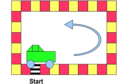
[image:3.595.328.520.203.341.2]drive around a track, which consists of 32 sections. The objective of this task is to complete 3 laps in the shortest amount of time. If a robot fails to complete 3 laps, the distance covered is the measure of its performance. The robot has to drive around the track covering all of the sections of the track, it is not allowed to skip any sections. In total the robot has to complete 3 laps, with 32 sections in each lap, all visited in the correct order. If the robot is too slow at driving between two sections the simulation is terminated. The following Fig. 1, illustrates the task to be completed:
Fig. 1. The figure illustrates the track and the robot in the simulator.
[image:3.595.397.451.470.582.2]Fig. 1 illustrates the track and the robot driving around it. The robot is not limited in its movement, i.e. it can drive off the track, reverse around the track or adapt to any driving patterns desired, as long at its drives over the right counter clockwise sequence of sections. The following Fig. 2 illustrates how the robot perceives the track and its environment.
Fig. 2. The figure illustrates the robot and its sensors.
Fig. 2 illustrates the robot driving on the track seen from above. The track sections have alternating colours to mark a clear distinction between sections. The arrows in Fig 2. illustrates the three sensors of the robot. The front sensor measures the distance to the next turn and the two side sensor measures the distance to the edge of the track. As indicated by Fig. 2, the simulated robot has three wheels and not four, to increase the difficulty of evolving a successful controller. The risk when driving this three wheeled robot, in contrast to a four wheeled vehicle, is that it will roll over if driven to abruptly. A robot that has rolled over is unlikely to be able to continue. The front wheel controls the speed as well as the direction.
V. EXPERIMENTS AND RESULTS
A total of three sets of experiments have been conducted. One reorganization takes place in two of the experiments. One set of experiments, with a randomly selected neural network, acts as a benchmark for further comparisons. This network only has its connection weights evolved, whereas the topology is fixed. One of the other set of experiments starts with the benchmark network selected in the first experiment, which is network then reorganized. This reorganization is only minor, in that only one connection is removed and replaced in each network. The new network resulting from the reorganization is tested. The third and final set of experiments also uses the network from experiment one as a starting condition. The network is then reorganized more extensively, by reshuffling several connections to create two new networks based on the old network. The results from these experiments are used to compare the different strategies of evolution.
A. The Simulation Environment
[image:4.595.65.272.426.587.2] [image:4.595.341.509.620.718.2]The evolved neural network controllers are tested in a physics simulator to mimic a real world robot subject to real world forces. The genetic algorithm has in all tests a population size of 50 and the number of tests per method is 15. Uniformly distributed noise has been added on the input and output values to simulate sensor drift, actuator response, wheel skid and other real world error parameters. The simulated robot can be seen in the following snapshot from the simulator:
Fig. 3. The figure illustrates the robot and the track in the simulator.
Fig. 3 shows a snapshot from the simulations. The robot, the wheeled box in the middle, is driving along the track, which is visualised by the rectangles of alternating colour. Fig. 3 is similar to Fig. 1 and it gives an idea of how the artificial neural network controllers simulated robot driving around a virtual track. To give the simulation similar attributes and effects as a on real racing track, the track has been given edges, which can be seen in Fig. 3. Whenever the robot drives off the track it falls off this edge onto another slower surface. This means, that if the robot cuts corners, it could potentially have wheels lifting off the ground thus affecting stability and speed, due to the edge coming back onto the track.
B. The Fitness Function
Fitness is rewarded according to normal motorsport rules and practice. 3 laps of the track have to be completed and the controller that finishes in the fastest time wins the race, i.e. it is the most fit controller. If a controller fails to finish 3 laps, the controller with the most laps or longest distance traveled wins. In the case that two controllers have reached the same distance the racing time determines the most fit controller. The fitness function can in general terms be described by the following:
Fitness
=
Distance Covered
Time
.
(3)The equation states that the longest distance covered in the shortest amount of time yields the best fitness. Time is the time it takes to complete the track. If a controller fails to finish this Time is set to 480 seconds, which is the absolute slowest a controller is allowed to be, before a simulation is stopped. In the likely event that to controllers have covered the same distance, the controller with the fastest time will be favored for further evolving. The precise version of the fitness function can be seen in the following:
Fitness
=
Sections
Laps
∗
Track Length
Time
.
(4)The fitness is equal to the distance divided by the time. The distance is equal to the number of track sections covered in the current lap, plus the number of sections covered in previous laps. Track length is the total number of sections, which is 32. The minimum fitness obtainable is 1/480 ≈ 0.002.
C. Initial Fixed Structure Network
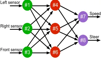
The first set of experiments conducted with a fixed structure network, where the connection weights were evolved, is used as the benchmark for the other experiments. This is the standard method of evolving artificial neural networks. The network used is a feed-forward connected network with three input neurons, 3 hidden layer neuron and two output neurons. The inputs are the sensor values as described previously and the outputs are the direction and speed of the front wheel. The network is shown in Fig. 4.
Fig. 4. The benchmark neural network.
This network was trained to competency and the results are shown in Table 1. The neural complexity of this network is 14.71, calculated with (2).
#1 #4
#5
#6
#8 #7
#2
#3
Left sensor
Right sensor
Front sensor
D. Minor Reorganization
[image:5.595.55.284.181.255.2] [image:5.595.311.543.186.321.2]The second set of experiments is conducted with a network that has been reorganized. The benchmark network has undergone a minor reorganization, which is shown in Fig. 5. The connection between neuron 6 and neuron 8 has been rearranged and is now a recursive connection. The new network has increased its neural complexity by the reorganization to 15.03.
Fig. 5. The first reorganized neural network.
Immediately after the reorganization the network loses some of its it fitness, this fitness is regained by retraining. The reorganized network was retrained with the same weights as before the reorganization and in all cases the network, as a minimum, regained all of its previous fitness and behavior. Additionally, all of the connection weights were re-evolved in another experiment to see if the results and tendencies were the same, and as expected the results were the same.
E. Major Reorganizations
[image:5.595.310.544.424.573.2]The final set of experiments conducted used a network, which has had a major reorganization. The benchmark network was changed by removing a connection between neuron 3 and 5 and between neuron 1 and 6. These connections are moved to between neuron 5 and 4 and between neuron 8 and 6. As the benchmark network is feed-forward connected only recursive connections are possible for this particular network. The new network is shown in Fig. 6.
Fig. 6. The second reorganized neural network.
The neural complexity of the new network has risen to 15.40, which is an 5% increase. Similar to the previously reorganized network, this network was, after a reorganization, subject to a fitness loss, but it was retrained to competency. The controller increased its fitness over the original network. Even re-evolving all of the connection weight yields a better overall performance.
F. Evaluation and Comparison of the Proposed Methods
The results from all of the experiment show that all networks learn the task proficiently, however some networks
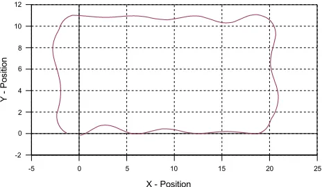
seem to perform better than others. Fig. 7 and Fig. 8 shows the route that controllers choose to drive around the track. The route reflects the results which are summarised in table 1. The race car starts in (0,0) and drives to (20,0) where it turns. Hereafter it continues to (20,11) where it turns and continues to (-2.5,11) and from here it continues to (-2.5, 0) and on to (0,0). The controller tries to align the car on the straight line between the points. Fig. 7 shows an average lap of the fixed structure networks, and it clearly illustrates the route that the car takes.
Fig. 7. The route of the fixed structure network.
[image:5.595.54.285.549.616.2]Fig. 7 illustrates how the fixed structure networks performs and the degree of overshoot when turning and recovering to drive straight ahead on another leg of the track. Fig. 8 shows the average route for the networks that have undergone a major reorganization.
Fig. 8. The severely reorganized neural network.
[image:5.595.306.545.711.789.2]The two figures shows the routes of the different networks. Fig. 8 clearly shows that the controllers that have been reorganized overshot less than the fixed structure networks in Fig 7. Less overshot, ultimately means that the racing car is able to move faster, which means it has a better fitness. The gathered results are summarised in the following table:
Table 1. Results from experiments Method Minimum
Fitness
Average Fitness
Maximum Fitness
Standard Deviation
Fixed Topology 0.857 0.964 1.042 0.062
Minor
Reorganisation 0.866 0.998 1.138 0.112
Major
Reorganisation 1.002 1.058 1.120 0.047
#2
#3
#1 #4
#5
#6 #8 #7
#2
#3
#4
#5
#6 #8 #7 Reorganisation #1
#2
#3
#1 #4
#5
#6 #8 #7
#2
#3
#4
#5
#6 #8 #7
Reorganisation #1 -10 0 10 20 30
-2 0 2 4 6 8 10 12
X - Position
Y
- Po
si
tio
n
-5 0 5 10 15 20 25
-2 0 2 4 6 8 10 12
X - Position
Y
Po
si
tio
The table shows the fitness from the fixed structure network experiments, and the fitness regained by the new networks after a reorganization and retraining.
The hypothesis that artificial neural networks that have undergone a minor reorganization, where the neural complexity is optimized, are statistically better than the fixed structure network it originates from does not hold true for these experiments. A t-test, with a 5% significance level, indicates that there is no statistical difference between the two methods, despite the higher minimum, average and maximum values. The second hypothesis tested in this paper, states that artificial neural networks that have undergone a major reorganization, again where the neural complexity is optimized, are better than the networks they originate from, holds true. A t-test, with a 5% significance level, indicates that there is a statistical difference between the two methods. This can be due to the increased neural complexity of the new network created by the reorganization. Some of this increased performance can possibly be accredited to the fact that one of the networks has a recursive connection, which is a common way to increase the neural complexity and performance of a network, but the experiments indicate that this is only part of the explanation. The experiment clearly indicates that increased neural complexity yield a higher probability of finding suitable and well performing neural networks, which is in line with other research in the field[14].
The results from the experiments doesn't indicate any significant difference in the speed of learning produced by either methodology. This means that it takes about the same number of iterations to learn a given task for any network topology used in the experiments, this was expected as they all have the number of parameters.
VI. CONCLUSION
This paper has presented a new methodology for complexifying artificial neural networks through structural reorganization. Connections were removed and reinserted whilst trying to increase the neural complexity of the network. The evolved neural networks learned to control the vehicle around the track and the results indicate the viability of the newly reorganized networks. The results also indicates that it might be necessary to rearrange more than one connection in order to achieve significantly better results. This paper indicates, that neural complexity in conjunction with reorganization can help unleash potential and increase the probability of finding neural network controllers of sufficient complexity to adequately solve complex tasks. Furthermore, the results indicate that a reorganization can substitute structural elaboration as a method for improving network potential, whilst keeping the computational overhead constant. These results are in line with previous research done in the field and they reconfirm the importance of high neural complexity and structural change.
REFERENCES
[1] A.S. Weigend, D.E. Rumelhart and B.A. Huberman, “Back-propagation, weight-elimination and time series prediction,”
Proceedings of the 1990 Summer School on Connectionist Models, 1990.
[2] J. Denker, D. Schwartz, B. Wittner, S. Solla R. Howard, L. Jackel and J. Hopfield, “Large Automatic Learning, Rule Extraction and Generalization,” Complex Systems, vol. 1, no. 5, 1987.
[3] S. Nolfi, and D. Floreano, Evolutionary Robotics; The Biology, Intelligence, and Technology of Self-Organizing Machines. MIT Press 2000.
[4] X. Yao and Y. Liu, “A New Evolutionary System for Evolving Artificial Neural Networks,” IEEE Trans. Neural Networks, vol. 8, no. 3, May 1997.
[5] X. Yao, “Evolving Artificial Neural Networks,” Proc. of the IEEE, vol. 87, no. 9, September 1999.
[6] R. Jacobs and M. Jordan, “Adaptive mixtures of local experts,”
Neural Computation, vol. 3, 1991.
[7] S. E. Fahlman, and C. Lebiere, “The Cascade-Correlation Learning Architecture,” Advances in Neural Information Processing Systems 2, Los Altos CA, US, 1990.
[8] T. Jorgensen, and B. Haynes, “Evolving Co-operative behavior,” in
Proc. of SAB06 Workshop on Bio-inspired Cooperation and Adaptive Behaviours in Robots, Rome 2006.
[9] P. Angeline, and J.Pollack, “Evolutionary Module Acquisition,” in
Proc. of the Second Annual Conf. on Evolutionary Programming, 1993.
[10] P. Angeline, G. M. Saunders, and J. B. Pollack, “An Evolutionary Algorithm that Constructs Recurrent Neural Network,” IEEE Trans. on Neural Networks, 1994.
[11] M. Lungarella, and O. Sporns, “Information Self-Structuring: Key Principle for learning and Development,” in Proc. of the fourth IEEE Int. Conf. on Development and Learning, 2005.
[12] O. Sporns, G. Tononi, and G. M. Edelman, “Connectivity and complexity: the relationship between neuroanatomy and brain dynamics,” in Neural Networks 13, 2000.
[13] O. Sporns, “Small-world connectivity, motif composition, and complexity of fractal neuronal connections,” in Biosystems 85, 2006. [14] O. Sporns, and M. Lungarella, “Evolving Coordinated Behaviours by
Maximizing Informational Structure,” in Proc. of the Tenth Int. Conf. on Artificial Life, 2006.
[15] K. O. Stanley, and R. Miikkulainen, “Continual Coevolution through Complexification,” in Proc. of the Genetic and Evolutionary Conference, 2002.
[16] G. Tononi, O. Sporns, and G. M. Edelman, “A Measure for Brain Complexity: Relating Functional Segregation and Integration in the Nervous System,” in Proc. of the National Academy of Science of USA, May 1994.
[17] L. S. Yaeger, and O. Sporns, ”Evolution of Neural Structure and Complexity in a Computational Ecology,” in Proc. of the Tenth Int. Conf. on Artificial Life, 2006.
[18] R. Dawkins, Climbing Mount Improbable. Reprint by Penguin Books, London, England 2006.
[19] G. N. Martin, Human Neuropsychology. Prentice Hall, 1998, Reprinted 1999.
[20] G. Edelman, Neural Darwinism – The Theory of Neuronal Group Selection. New York:Basic Books, 1989, Print by Oxford Press 1990. [21] C. E. Shannon, “A Mathematical Theory of Communication,” The