Abstract—A localization method for a mobile robot moving in outdoor environment near buildings is presented in this paper. The localization method utilizes Particle filtering with index function based on Normal Distributions Transform (NDT) algorithm. In the proposed method, the robot position is estimated by comparing horizontal scan data with the 2D map extracted from 3D map. For that, a 3D map is made by using a 3D scan device equipped on the mobile robot firstly. Then it is converted to a 2D map for localization by extracting point data in a certain range of height. Experiments of mapping and localization in outdoor area near buildings were demonstrated.
Index Terms— mobile robot, mapping, 3D scan, localization, NDT algorithm
I. INTRODUCTION
ECENTLY, the development of robot technology is remarkable. Its rapid progress is leading to expansion of robotics application area, especially in daily environments. The automatic driving technology for unmanned vehicle is one of its representative examples, which is related to mobile robot. For the case of a mobile robot, a capability of autonomous navigation is essential. The process for robot navigation includes four general steps as follows; making map, localizing in the map, planning a path to a goal position, and controlling the robot to follow the path. Hence a map is used as a fundamental tool for autonomous navigation because the position of the robot is defined on it.
2D map that has been used widely in accordance with recent rapid advance of laser scanner, is a well-known effective tool for indoor navigation. Many approaches of localization using 2D map have been investigated for the robot navigation in indoor environments [1, 2, 3].The position of the robot is estimated by comparing current 2D scan data with a map. For the method of comparing, Iterative Closest Point (ICP) algorithm has been used widely. Meanwhile, for outdoor environment, there are other researches of localization utilizing 3D map [4, 5, 6]. Generally, Global Positioning System (GPS) is absolutely an easy and simple method for estimating the current robot position in outdoor environment. There are many researches of localization using GPS in outdoor environment [7, 8]. However, when the robot moves
Manuscript received December 8, 2015; revised January 20, 2016. This work was supported by Okumuragumi Research Fund.
Every author is with Mechanical Engineering Corse, Graduate School of Science and Engineering, Ehime University, 3 Bunkyo-Cho, Matsuyama 790-8577, Japan.
E-mail: Shohei Kita <[email protected]> Jae Hoon Lee <[email protected]>
Shingo Okamoto <[email protected]>
near or between buildings, the position given from GPS has fatal error due to bouncing off the buildings. In addition, localizing method based on 2D map is also not effective because the robot’s posture cannot be kept horizontally due to unevenness of the terrain in outdoor environment.
There are other methods of localization using 3D scan data with a 3D map. For this case, the position and posture of the robot can be estimated. However, it requires a long time for calculation of matching 3D scan data. The amount of 3D scan data is greater than that of 2D scan, thus most scan matching algorithms such as ICP require computing power to find correspondences between the map and the current scan data. So it needs particular method that can reduce calculation time to estimate the position of the robot effectively. In order to solve the problem, Biber proposed NDT algorithm [9]. Similar to an occupancy grid, the NDT makes a regular subdivision of plane and the NDT models the distribution of all reconstructed 2D points by collection of local normal distribution. In addition, the NDT represents the probability of measuring a sample at 2D point for each position within the cell. In general matching algorithm, the correspondence point is found by comparing each scan point with all map points. However, by using the NDT, the algorithm searches in which cell the scan data should be corresponded. Moreover, the correspondence can be easily calculated by using the mean and probability of the cell. So, it is expected that the calculation time could be reduced because the process of finding correspondence is carried out in each cell. Newton’s algorithm is used for the optimization process of the NDT algorithm. However, in case of Newton’s algorithm, there is particular problem near local minimum where the eigenvalue of covariance matrix is changed largely.
In order to solve the above-mentioned problem, a method to estimate the robot position utilizing Particle filter [10] and NDT algorithm has been considered in this paper.
Experiments of NDT-Based Localization
for a Mobile Robot Moving Near Buildings
Shohei Kita, Jae Hoon Lee , Member, IAENG and Shingo Okamoto
R
(a) Mobile robot system (b) 3D scan device
IMU Senso r
LRF Servo
Motor
Encoder Encoder
3D Scan Device
By using the algorithm, it is expected that the calculation time could be reduced and more accurate position also could be achieved. In order to check the effectiveness, experiments of localization has been performed by using a mobile robot in outdoor environment near buildings.
II. MOBILE ROBOT SYSTEM
A. System Configuration
Fig. 1 shows the mobile robot that had been developed in this research. Fig. 2 shows the system configuration of the robot [11]. The 3D scan device on the robot consists of a Laser Range Finder (LRF) sensor, a servo motor for rotating the LRF in pitch direction and an encoder to measure the pitch angle. A laser scanner (UTM-X001s, HOKUYO AUTOMATIC CO., LTD.), whose angular resolution is 0.25 [deg] and measurement distance is 0.1 [m] to 30 [m], has been used as the LRF sensor. Its field of view is 270 [deg]. The resolution of pitch angle which is measured by the encoder is 0.09 [deg].
LRF sensor scans the horizontal plane and provides continuously the range data and the yaw angle for each scan point. When the LRF is tilted by using the servo motor iteratively, the pitch angle of each scan plane is changed. Then, the multiple scan data of the scan planes are given with their pitch angles. Resultantly they becomes a cloud of 3D points and their positions also can be computed with pitch and yaw angle information. Here, Inertial Measurement Unit (IMU) sensor is used to measure the posture of the robot. In addition, the position of robot is estimated by using the encoders equipped at both wheels.
All devices and embedded controller are connected to the main controller. The laptop computer of Intel Core i7-4510U 2.0 [GHz] with Linux OS of Ubuntu 14.04 was used as the main controller in this research.
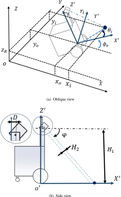
B. Coordinate Transformation
The position of each scan point is computed based on the coordinate transform as follows. Its schematic representation is displayed in Fig. 3. The parameters for the coordinate transformation are defined below.
: Global coordinate system
: Moving coordinate system attached to the robot center, i.e. center position of both wheels
:Coordinate of the i-th scan point with respect to the moving coordinate system
:Coordinate of the i-th scan point with respect to the global coordinate system Z
:Distance from the LRF to an object in i-th scan point :Yaw angle of i-th scan point
:Pitch angle of i-th scan point
:Distance from the center of both wheels to LRF in direction
:Height from the ground to the axis of the servo motor for tilting motion
:Height from emitted point of infrared ray of LRF to axis of rotation of the servo motor
:Coordinate of the robot position in the global coordinate
:Posture angle in the manner of Euler angle method around the each axis
The position and posture in global coordinate is measured from odometry. However, measurement error can be occurred in odometry information due to wheel slip, terrain condition and so on. So, it is necessary to be considered for matching. The robot position and pose in the planar space can
Fig. 2. Configuration of the mobile robot system with 3D scan device
(b) Side view
[image:2.595.306.548.285.680.2] [image:2.595.49.289.499.649.2]be defined with the odometry information, , and the error, , as following equations.
(1)
(2) (3) The coordinate of i-th scan point with respect to the moving coordinate system fixed to the robot is given by
(4) Where and denote and , respectively.
The posture of the mobile robot is changed according to the slope or the unevenness of road terrain. Therefore, the coordinate of i-th scan point in the moving coordinate should be converted into the global coordinate. Here, the posture of the robot is defined as .Also, the yaw angle, , includes both rotations due to the usual robot motion and the terrain condition. Thus it is given by Eq. (5).
(5) The coordinate of i-th scan point in the global coordinate is given by Eq. (6).
(6)
III. MAPPING
A. Matching process for making 3D map
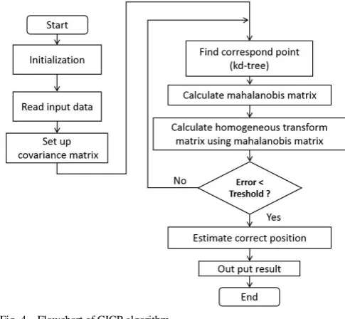
A map in this paper is made by accumulating scan data which measured by 3D scan device equipped on the robot. However, the measured data includes errors due to uncertainty of sensor itself, slipping of the wheels on the ground, synchronization problem between sensors in random motion of the robot and so on. For reducing the errors, a matching algorithm to align two sets of point clouds has been used for matching process. ICP algorithm is widely used as matching method for that [12]. In ICP algorithm, a homogeneous transform matrix that matches a scan data to a reference data is utilized. Then, the most important process is how to estimate the homogeneous transform matrix based on the correspondences between two clouds of scan points.
In this paper, Generalized Iterative Closest Point (GICP) algorithm which was developed by Aleksandr V. Segal has been used for matching process [13]. The time for searching the correspondence points is reduced by using the kd-tree algorithm [14]. Moreover, the correspondence between the
scan data and the reference data is calculated by Mahalanobis distance instead of Euclidean distance. Then, the homogeneous transform matrix is computed as the optimal solution so that the square sum of the Mahalanobis distance of correspondence points is minimized. The position and posture are estimated by these processes, iteratively. Fig.4 shows the flowchart of GICP algorithm.
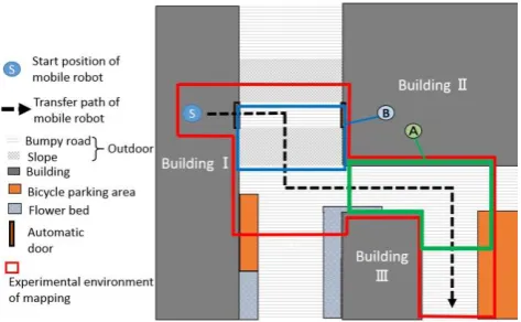
The map building had carried out in the outdoor environment near buildings. The schematic map and the area of mapping are shown Fig. 5. Where the trajectory of the robot during 3D scanning is depict with the dashed line which starts from ‘S’ position. All 3D scan data was measured by manner of ‘move and stop for scanning.’ Namely, the robot is stopped while the 3D scanning is being carried out. Then, the robot moved again to the next scanning position after the 3D scanning was finished. The 3D scanning had been performed for every time that the robot had been moved 3 meters.
[image:3.595.54.291.184.259.2]After all 3D scanning, its off-line matching process had been carried out with GICP algorithm. At first, the 3D data obtained at the start position is used as the reference data. The 3D data obtained in the next position is matched to the reference data. Then, the matched data becomes a new reference data, and the next scan data is registered after matching process. These processes are carried out iteratively until finishing to match all scan data. The top view of the resultant 3D map achieved in the experiment is displayed in Fig. 6.
B. Method for making 2D map
For estimating the robot position in the outdoor environment near buildings, 2D map-based localization method has been employed in this research. Generally 2D map is made by matching multiple 2D scan data. However, in the case of outdoor navigation, it is difficult to match them correctly owing to differences between multiple scan data. The reason is fundamentally based on the fact that the scan data for the horizontal plane of certain height cannot be achieved always. In addition, the change of the robot’s position due to slippage of the wheels and the unevenness of
[image:3.595.314.557.402.626.2]road terrain cannot be detected with 2D scan data. Moreover, the 2D scan data is inclined due to this problem. In the case of 2D map data consisting of only horizontal plane whose height is the same one as the laser scanner on the robot, the 2D scan data cannot be matched with the 2D map because the inclined 2D scan data is different from the horizontal plane of the 2D map. Therefore, the problem deteriorate matching performance.
In order to cope with the problem, the map for localization was extracted from a 3D map including horizontal plane with terrain shape also. Firstly, a 3D map is made by GICP algorithm as matching method [13]. After then, the data included in the horizontal plane, whose height is the same of the laser scanner on the robot, is extracted as the 2D map for localization because the robot use the horizontal scan data for estimating the position of itself. The center of the horizontal plane is positioned at the height of 1044 [mm] and its range is defined as 600 [mm], respectively.
IV. LOCALIZATION
A. Method of NDT-based localization
The simple idea to find the current position where a scanning was done is to compare the data with map data and find the optimal position fitting with each other. However, in the case of localization in wide area, it requires long time for comparing them because the amount of the map data is extremely large. Besides, the computation cannot be done in real time for some cases.
For reducing the calculation time, the NDT algorithm is used in this research. It is similar to an occupancy grid. It
establishes a regular subdivision of the planar space and represents the probability of measuring a sample for each position within the cell. Generally, in order to estimate the position of the robot, the correspondence point is obtained by comparing the scan point with all points of map data. However, in the case of the NDT, the correspondence is obtained by comparing scan points with the probability and mean within the cell. So, the calculation time of matching process is reduced because the computation of correspondence is carried out in each cell and the scan point could be assigned to its cell straightforwardly without finding process.
The NDT algorithm includes following processes. At first, the 2D map data is subdivided regularly into the cells with constant size. A cell size is defined as a square of 500 [mm] by 500[mm] in this research. Then, the mean and covariance of are prepared for each cell with the data in it. Thirdly, the correspondence for the scan data at the current robot position is computed. Here, the normal distribution is calculated with the scan data and the map, i.e., the covariance matrix and mean. Finally, the sum of the normal distribution is calculated by the following equation.
i
i i t i
i q i p q
p E
2 exp
1
(7)
Here, pi denotes 2D scan point data measured by using LRF of i-th cell, qidenotes the mean which calculated from map data of i-th cell, and the covariance matrix which calculated from the mean and the scan data of i-th cell is defined as , respectively.
In the case of the original NDT localization [9], the current robot position is estimated by optimization process. However, Particle filter [10] instead of optimization has been used for estimating the current position in this research.
For the Particle filter, the motion model of the robot is defined by the following equation.
T r r
r r v
l l r r
l l r r
R R
/ 2 /
(8)
Here, thevR and
Rdenote the translational and rotational velocities of the mobile robot, respectively. The r andl
denote the rotational velocities of each wheel, respectively. Therrand rl denote radii of each wheel, respectively. Then the width of the mobile robot is denoted as T.
The posture of the robot at time k is known as
TR R Rk y k k x
k
R . Here,
xR
k yR
k
Tdenotes the position of the coordinates on the map and R
k denotes the posture of the robot. Then, the posture of the robot at time1
k is given as follows. The tdenotes infinitesimal time between k andk1.
[image:4.595.52.289.286.432.2]
t t k v t k v k k y k x k k y k x R R R R R R R R R R R sin cos 1 1 1 (9)The particles are made by supplying the rotational velocity of each wheel with random numbers as uncertainties of model and measurement. By using this method, the particles can be propagated according to the motion model. The random number is calculated by using Box-Muller’s method.
The weight of each particle is calculated by using the sum of the normal distribution indicated by Eq. (7). The weight of b-th particle is given by Eq. (10).
p j j b
b E E
w / 0 (10)
Here, Ebdenotes the sum of the normal distribution of b-th particle, and the sum of the normal distribution of all particles is denoted as pj0Ej, respectively.
Resampling is carried out by the following process. Firstly the particles of forty percent with small weights in all ones are deleted. Then the particles with the same number as the deleted ones are made using the ones with large weights in the remaining ones. Consequently the total number of particles are kept in the initial one.
Resultantly, the posture is estimated by the weighted mean of particles.
By repeating these process, the posture of the robot is estimated so that the sum of the normal distribution can be increased.
B. Method for experimental works
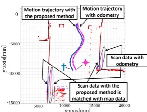
The experiments of localization had been carried out in the outdoor environment near buildings of Engineering Faculty in the campus of Ehime University. The areas for the experiments were depicted as ‘A’ and ‘B’ in Fig. 5. The robot moved with sinusoidal trajectory in both areas. While moving, the robot scans horizontal plane and its odometry information is also saved at the same time. Where one scan data per every 30 times of scanning was used for localization process. The localization process had been carried out off-line by using the proposed method. The resultant position was compared with the odometry information.
C. Experimental results
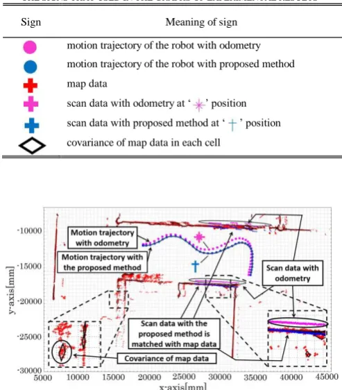
The experimental environment of area ‘A’ and ‘B’ are shown in Fig. 7 and Fig.9, respectively. The experimental results of localization in the area of ‘A’ and ‘B’ are shown in Fig. 8 and Fig. 10, respectively. Where the signs used in experimental results are shown in TABLE I. In the case of area ‘A’, the condition is similar to an indoor environment but includes a bicycle parking place. Besides, it is observed that the map data has ambiguous part on the wall of Building III. It is owing to many small holes on the wall of the right building in Fig. 7 (a). In spite of the uncertain condition in the map, the proposed method could estimate the robot position in the area of ‘A’ well resultantly as shown in Fig. 8. In the case of the area ‘B’ of Fig. 9, the road has the slope part from the building door to outside. When the position of the robot is estimated by odometry, an accumulative error is occurred due to the slippage of wheels and the unevenness of road terrain and so
on. Especially it becomes large for moving long distances. However, by using proposed method, the correct position of the robot could be estimated even in the slope as shown in Fig. 10.
(a) Photograph of the area between buildings which was taken from the building I side.
(b) Photograph of the corner in area ‘A’ which was taken from the building II side. Fig. 7. The area ‘A’ of experimental environment
TABLEI
THE SIGNS THAT USED IN THE GRAPHS OF EXPERIMENTAL RESULTS
Sign Meaning of sign motion trajectory of the robot with odometry motion trajectory of the robot with proposed method map data
scan data with odometry at ‘ ’ position scan data with proposed method at ‘ ’ position covariance of map data in each cell
[image:5.595.305.550.111.247.2] [image:5.595.306.550.276.454.2] [image:5.595.302.549.492.773.2]V. CONCLUSIONS
It has been known that the typical odometry has accumulation error for long distance movement. Moreover, it is more severe in case of outdoor environment because robot wheels may slip due to the unevenness of the outdoor terrain. To solve this problem, the robot localization method with NDT map was investigated in this paper. In this method a 2D map is extracted from the 3D map data that was obtained by using a 3D scan device installed on the mobile robot. In the 2D map there are some ambiguous conditions such as many small holes on the building wall which prevent high matching accuracy. Solving this problem, the Particle filter with NDT was adopted.
As a result, by using the proposed method, the robot position was estimated experimentally with high accuracy than typical odometry method. By using the odometry, the error of the estimation position increased, as the movement distance increased. On the other hand, by using the proposed method, the error is smaller than that of odometry. Overall, however, the correct position of the robot could be estimated. Moreover, in the case of off-line experiments, when 100 particles were used, the calculation time is 0.09 [sec] for one positioning. So, in the case of on-line experiment, it is expected that the estimation could be performed in real time.
REFERENCES
[1] K. Konolige, G. Grisetti, R. Kummerle, W. Burgard, “Efficient Sparse Pose Adjustment for 2D Mapping,” Proceedings of 2010 IEEE/RSJ International Conference on Intelligent Robots and Systems, pp. 22-29, 2010.
[2] J. Miura, Y. Negishi, Y. Shirai, “Mobile Robot Map Generation by Integrating Omnidirectional Stereo and Laser Range Finder,”
Proceedings of 2002 IEEE/RSJ International Conference on Intelligent Robots and Systems, pp. 250-255, 2002.
[3] A. Oliver, S. Kang, B. C. Wunche, B. Macdonald, “Using the Kinect as a Navigation Sensor for Mobile Robotics,” Proceeding of the 27th Conference on Image and Vision Computing New Zealand, pp. 509-514, 2012.
[4] M. Bosse, R. Zlot, P. Flick, “Zebedee: Design of a Spring-Mounted 3-D Range Sensor with Application to Mobile Mapping,” IEEE Transactions on Robotics, vol. 28, pp. 1104-1119, 2012.
[5] R. Valencia, E. H. Teniente, E. Trulls, J. Andrade-Cetto, “3D mapping for urban service robots,” Proceedings of 2009 IEEE/RSJ International Conference on Intelligent Robots and Systems, pp. 3076-3081, 2009. [6] A. Nüchter, K. Lingemann, J. Hertzberg, H. Surmann, “6D SLAM-3D
mapping outdoor environments,” Journal of Field Robotics, vol. 24, pp. 699-722, 2007.
[7] M. Agrawal, K. Konolige, “Real-time Localization in Outdoor Environments using Stereo Vision and Inexpensive GPS,” Proceeding of 18th International Conference on Pattern Recognition, pp. 1051-1068, 2006.
[8] T. Suzuki, M. Kitamura, Y. Amano, T. Hashizume, “6-DOF localization for mobile robot using outdoor 3D voxel maps,”
Proceedings of 2010 IEEE/RSJ International Conference on Intelligent Robots and Systems, pp. 5737-5743, 2010.
[9] P. Biber, W. Strasser, “The Normal Distributions Transform: A New Approach to Laser Scan Matching,” Proceedings of 2003 IEEE/RSJ International Conference on Intelligent Robots and Systems, pp. 2743 - 2748, 2003.
[10] D. Fox, S. Thrun, W. Burgard, F. Dellaert, “Particle Filters Mobile Robot Localization,” Sequenrial Monte Carlo Methods in Pratice Part of the series Statistics for engineering and Information Science, pp. 401-428, 2001.
[11] K. Hayashida, J. H. Lee, S. Okamoto, “A method to recognize road terrain with 3D scanning,” Ubiquitous Robots and Ambient Intelligence, pp. 432-436, 2011.
[12] P. Besl, N. McKay, “A Method for Registration of 3-D Shapes,”
Proceedings of IEEE International Conference on Pattern Analysis and Machine Intel, vol. 14, pp. 239-256, 1992.
[13] Aleksandr V. Segal,Dirk Haehnel and Sebastian Thrun, “Generalized-ICP,” Robotics Science and System, 2009.
[image:6.595.48.296.59.204.2][14] Z. Zhang, “Iterative Point Matching for Registration of Free-FormCurves,” IRA Rapports de Recherche, Robotique, Imageet Vision, pp. 1658, 1992.
[image:6.595.46.283.235.416.2]