Repetitive Sampling
Gadde Srinivas Rao
Department of Statistics, School of Mathematical Sciences, CNMS, The University of Dodoma, Dodoma, PO. Box: 259, Tanzania. [email protected]
Muhammad Aslam
Department of Statistics, Faculty of Science, King Abdulaziz University, Jeddah 21551 [email protected]
Muhammad Azam
Department of Statistics and Computer Science,
University of Veterinary and Animal Sciences, Lahore 54000, Pakistan [email protected]
Chi-Hyuck Jun
Department of Industrial and Management Engineering, POSTECH, Pohang 790-784, Republic of Korea [email protected]
Abstract
In this manuscript, a control chart is designed for two-piece normal distribution using repetitive sampling. The necessary measures to determine the average run lengths for in control and out-of-control process are given. The average run lengths are presented for various specified parameters and shift constants. The efficiency of the proposed chart is compared with the existing control chart using single sampling. The application of the proposed chart is given with the help of an example.
Key words
Two-piece normal distribution; control chart; repetitive sampling; average run length
1. Introduction
Statistical analysis plays an important role in the production of high quality product. Among them, a control chart is a useful tool to monitor the manufacturing process. It is used to indicate when the process is going to be out-of-control. Usually, a control chart is based on two natural limits called upper control limit (UCL) and lower control limit (LCL). The process beyond these limits is called out-of-control process. The manufacturing process can be shifted due to some controllable and uncontrollable factors. Due to the shift, the process can be away from the given specifications limit and results in non-conforming products. A quick indication about the out-of-control state helps to minimize the rework and non-conforming product.
always follows the normal distribution. In this situation, the use of a control chart based on normal distribution assumption increases the false alarms. So, it is necessary to develop control charts designed for normal distributions. The details about non-normal control chart can be seen in Santiago and Smith.(2013), Amin et al., (1995) Bai and Choi (1995),Chang and Bai (2013), Al-Oraini et al.,(2002),Riaz et al.,(2014), McCracken, and Chakraborti (2013). The two-piece normal distribution is widely used when data is not symmetric. According to Britton and Fisher (1998) the two-piece normal distribution is used for this type of data. Kimber and Jeynes (1987) used this distribution in measurement of depths of arsenic implants in silicon. Simionescu (2014) used for fan chart to assess uncertainty.
By exploring the literature, we note that there is no work on designing a control chart for two-piece normal distribution. In this paper, we focus on the development of control charts for two-piece normal distribution using single and repetitive sampling. We will present the structure of proposed chart and compared the efficiency of the proposed charts. A simulation study is given for illustration of the proposed chart.
2. Design of Proposed Chart
A random variable, Z, has a two-piece normal (TPN) distribution with parameters (μ, σ1,
σ2) if it has the probability density function of
𝑓(𝑧) = {𝐴 𝑒 −(𝑧−𝜇)2
2𝜎12 ; 𝑧 ≤ 𝜇
𝐴 𝑒− (𝑧−𝜇)2
2𝜎22 ; 𝑧 ≥ 𝜇
(1)
Where 𝐴 = [√2𝜋 (𝜎1+𝜎22 )]−1 John (1982) shows the following relations for average and variance
𝜇𝑧 = 𝜇 + (𝜎2− 𝜎1)√2𝜋 (2) 𝜎𝑧2 = (1 −2
𝜋)(𝜎2− 𝜎1) 2+ 𝜎
1𝜎2. (3)
In the case of equal standard deviations (𝜎1 = 𝜎2) it will be a classical normal distribution, which is symmetric.
We propose the following Z-chart using repetitive sampling based on the statistic Z by following Aslam et al (2014) and Lee et al., (2014)
Step 1: Select an item randomly at each subgroup and measure its quality characteristic Z.
Step 2: Declare the process as out-of-control if 𝑍 ≥ 𝑈𝐶𝐿1𝑜𝑟 𝑍 ≤ 𝐿𝐶𝐿1. Declare the process as in-control if 𝐿𝐶𝐿2 ≤ 𝑍 ≤ 𝑈𝐶𝐿2. Otherwise, go to Step 1 and repeat the process.
The operational procedure of proposed chart is based on four control limits and two control chart coefficients. The limits LCL1 and UCL1 are called the inner control limits
and the limits LCL2 and UCL2 are called the outer control limits. As mentioned by Aslam
et al.,(2014)“the proposed control chart does not make a conclusion on the process state if the statistic lies between the inner and outer control limits, in which case repetitive sampling is required.
Let us assume that the outer control limits for the proposed control chart are symmetrically given by
LCL1 = μz− k1σz = 𝜇0+ (𝜎2− 𝜎1)√𝜋2− k1√(1 −2
𝜋)(𝜎2− 𝜎1)2+ 𝜎1𝜎2 (4)
UCL1 = μz+ k1σz = 𝜇0+ (𝜎2− 𝜎1)√𝜋2+ k1√(1 −2
𝜋)(𝜎2− 𝜎1)2+ 𝜎1𝜎2. (5)
where 𝜇0 is the parameter 𝜇when the process is in control. Also, the inner control limits for the proposed control chart are designed by
LCL2 = μz− k2σz = 𝜇0+ (𝜎2− 𝜎1)√𝜋2− k2√(1 −2
𝜋)(𝜎2− 𝜎1)2+ 𝜎1𝜎2 (6)
UCL2 = μz+ k2σz = 𝜇0+ (𝜎2− 𝜎1)√𝜋2+ k2√(1 −2
𝜋)(𝜎2− 𝜎1)2+ 𝜎1𝜎2. (7)
Note that k1 and k2 control limits coefficients and will be determined through simulation
later.
For the proposed control chart, the process is declared to be out-of-control if 𝑍 ≥ 𝑈𝐶𝐿1𝑜𝑟𝑍 ≤ 𝐿𝐶𝐿1. According to the parameterization by Banerjee and Das (2014), for single sampling, the probability that process is declare out of control when actually in control is denoted by 𝑃𝑜𝑢𝑡,10 and is given by
𝑃𝑜𝑢𝑡,10 = 𝑃{𝑍 ≤ 𝐿𝐶𝐿
1|𝜇 = 𝜇0} + 𝑃{𝑍 ≥ 𝑈𝐶𝐿1|𝜇 = 𝜇0} = 1 − 𝑃{𝐿𝐶𝐿1 < 𝑍 < 𝑈𝐶𝐿1|𝜇 = 𝜇0}
= 1 − 2𝜎1
𝜎1+𝜎2[𝜎2Φ ( 𝑈𝐶𝐿1−𝜇0
𝜎2 ) − 𝜎1Φ (𝐿𝐶𝐿1−𝜇0𝜎1 ) +𝜎1−𝜎22 ] (8)
The probability of repetition (𝑃𝑟𝑒𝑝0 ) for the proposed control chart is given as follows 𝑃𝑟𝑒𝑝0 = 𝑃{𝑈𝐶𝐿2 ≤ 𝑍 ≤ 𝑈𝐶𝐿1|𝜇 = 𝜇0} + 𝑃{𝐿𝐶𝐿1 ≤ 𝑍 ≤ 𝐿𝐶𝐿2|𝜇 = 𝜇0}
= 2𝜎1 𝜎1+𝜎2[𝜑 (
𝑈𝐶𝐿1−𝜇0
The probability that the process is out of control when actually under the repetitive sampling. it is in control is denoted by 𝑃𝑜𝑢𝑡0 and is defined as follows
𝑃
𝑜𝑢𝑡0=
𝑃𝑜𝑢𝑡,101−𝑃𝑟𝑒𝑝0 . (10)
The performance of proposed chart will be measured using the average run length (ARL) criteria. The ARL is used to indicate when on the average process will be out-of-control. The ARL when the process is in control is denoted by ARL0 and defined as follows
𝐴𝑅𝐿0 = 𝑃1
𝑜𝑢𝑡0 . (11)
Suppose now that the process parameter 𝜇is shifted to 𝜇1. Then, the probability of the process being declared to be out-of-controlbased on the single sample when the process is shifted is
𝑃𝑜𝑢𝑡,11 = 𝑃{𝑧 ≤ 𝐿𝐶𝐿
1|𝜇 = 𝜇1} + 𝑃{𝑧 ≥ 𝑈𝐶𝐿1|𝜇 = 𝜇1} = 1 − 𝑃{𝐿𝐶𝐿1 < 𝑧 < 𝑈𝐶𝐿1|𝜇 = 𝜇1}
= 1 − 2𝜎1
𝜎1+𝜎2[𝜎2𝜑 ( 𝑈𝐶𝐿1−𝜇1
𝜎2 ) − 𝜎1𝜑 (𝐿𝐶𝐿1−𝜇1𝜎1 ) +𝜎1−𝜎22 ] (12)
Similarly, the probability of resampling for shifted process is given as follows 𝑃𝑟𝑒𝑝1 = 𝑃{𝑈𝐶𝐿
2 ≤ 𝑧 ≤ 𝑈𝐶𝐿1|𝜇 = 𝜇1} + 𝑃{𝐿𝐶𝐿1 ≤ 𝑧 ≤ 𝐿𝐶𝐿2|𝜇 = 𝜇1} = 2𝜎1
𝜎1+𝜎2[𝜑 ( 𝑈𝐶𝐿1−𝜇1
𝜎2 ) − 𝜑 (𝑈𝐶𝐿2−𝜇1𝜎2 ) + 𝜑 (𝐿𝐶𝐿2−𝜇1𝜎1 ) − 𝜑 (𝐿𝐶𝐿1−𝜇1𝜎1 )] (13) So, the probability of the process being declared to be out of control (𝑃𝑜𝑢𝑡1 ) for the proposed control chart when the process is shifted is given as follows:
𝑃
𝑜𝑢𝑡1=
𝑃𝑜𝑢𝑡,111−𝑃𝑟𝑒𝑝1 . (14)
The out of control ARL for the shifted process is given as follows: 𝐴𝑅𝐿1 = 𝑃1
𝑜𝑢𝑡1 . (15)
According to Aslam et al.,(2014) “the proposed control chart requires re-sampling when the decision has not been made from the previous sample. The average sample size (ASS) is the expected number of resampling (or sample size) required until the final decision is made, and it can be used as one of the performance measures”. The average sample size for the in-control process (ASS0) and the shifted process (ASS1) is respectively given by
𝐴𝑆𝑆0 =1−𝑃1
𝑟𝑒𝑝0 (16)
𝐴𝑆𝑆1 =1−𝑃1
𝑟𝑒𝑝1 . (17)
Let r0 be the target in-control ARL. The following algorithm will be used to determine
the ARLs values.
1. Select the initial values of k1 and k2.
2. Generate a random variable at each subgroup from the two-piece normal distribution having the specified parameters for in-control process, that is, 𝜇0=0 and different values of 𝜎1 < 𝜎2 and 𝜎1 > 𝜎2.
the process is declared as out-of-control, record the number of subgroups so far as the in-control run length.
4. Repeat Steps 1-3 a sufficient number (10,000 say) of times to calculate the in-control ARL. If the in-control ARL is equal to the specified ARL0( say𝑟0 ), so as minimize ASS0 such that 𝐴𝑅𝐿0 ≥ 𝑟0then go to Step 5 with the current values of k1 and k2.
Otherwise, modify the values of k1 and k2 andrepeat Steps 2-4.
5. Then using Eq. (15), we obtain ARL1 based on the determined values of k1 and k2 for
various shift values of 𝜇1 = 𝜇0 + 𝛿𝜎1(𝜎1 < 𝜎2).
Table 1shows the ARLs according to the shift value𝛿 = 0.0 𝑡𝑜 2.0 with the interval of 0.1 whenr0 is 200 or 250, while Table 2reports on the ARLs when r0 is 300 or
370.Whereas, Tables 3 and 4 obtained the ARL1 values based on the determined values
of k1 and k2 for various shift values of 𝜇1 = 𝜇0− 𝛿𝜎1(𝜎1 > 𝜎2 ) according to the shift value 𝛿 = 0.0 to 2.0 with the interval of 0.1. From Tables 1, 2, 3 and 4, we note the following behavior of ARL1.
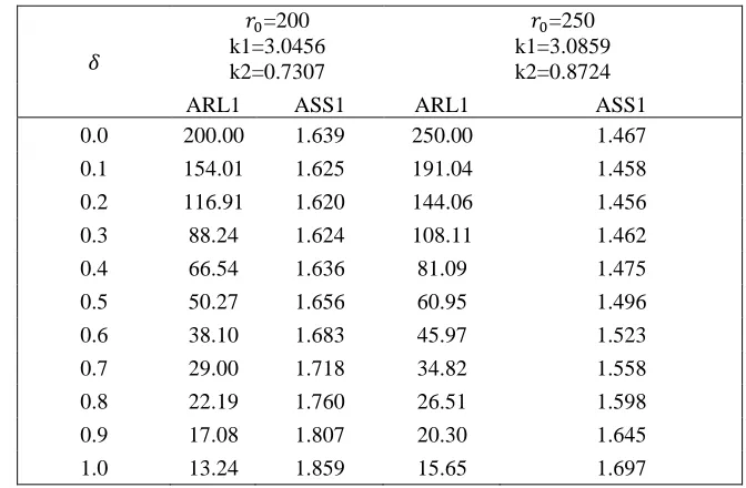
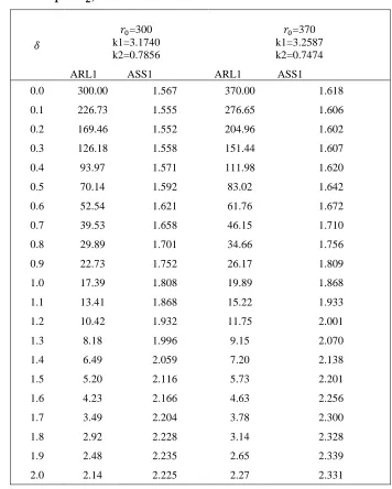
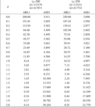
1. The case of 𝜇1 = 𝜇0 = 0, corresponds to the in-control ARL, which is obtained very close to the target r0 values.
2. As the shift 𝛿 increases (the process mean increases), the out-of-control ARLs decrease rapidly when 𝜎1< 𝜎2. Similar trend can be observed from Tables 3 and 4 when 𝜎1 > 𝜎2 whereas decreasing speed seems to get faster in the later case.
3. The decreasing speed in ARLs seems to get faster as r0 increases. The average sample
size for the out of control process (ASS1) increases as shift 𝛿 increases in both case
( 𝜎1 < 𝜎2or 𝜎1 > 𝜎2) .
4. The control constant k1 increases as r0 increases, while k2not follows this tendency
according to different r0’s when 𝜎1 < 𝜎2whereas control constant k2 increases as r0
increases in case of 𝜎1> 𝜎2, while k1 not follows this tendency according to different
r0’s.
Table 1: Average run lengths for proposed control chart when r0 is 200 or 250 ( when𝝈𝟏< 𝝈𝟐).
𝛿
𝑟0=200
k1=3.0456 k2=0.7307
𝑟0=250
k1=3.0859 k2=0.8724
ARL1 ASS1 ARL1 ASS1
0.0 200.00 1.639 250.00 1.467
0.1 154.01 1.625 191.04 1.458
0.2 116.91 1.620 144.06 1.456
0.3 88.24 1.624 108.11 1.462
0.4 66.54 1.636 81.09 1.475
0.5 50.27 1.656 60.95 1.496
0.6 38.10 1.683 45.97 1.523
0.7 29.00 1.718 34.82 1.558
0.8 22.19 1.760 26.51 1.598
0.9 17.08 1.807 20.30 1.645
1.1 10.34 1.915 12.15 1.752
1.2 8.15 1.971 9.51 1.811
1.3 6.48 2.027 7.52 1.870
1.4 5.22 2.079 6.00 1.927
1.5 4.25 2.124 4.85 1.980
1.6 3.51 2.159 3.97 2.026
1.7 2.94 2.182 3.29 2.061
1.8 2.50 2.189 2.77 2.084
1.9 2.16 2.181 2.37 2.092
2.0 1.89 2.156 2.05 2.084
Table 2. Average run lengths for proposed control chart when r0 is 300 or 370 ( when 𝝈𝟏< 𝝈𝟐).
𝛿
𝑟0=300
k1=3.1740 k2=0.7856
𝑟0=370
k1=3.2587 k2=0.7474
ARL1 ASS1 ARL1 ASS1
0.0 300.00 1.567 370.00 1.618
0.1 226.73 1.555 276.65 1.606
0.2 169.46 1.552 204.96 1.602
0.3 126.18 1.558 151.44 1.607
0.4 93.97 1.571 111.98 1.620
0.5 70.14 1.592 83.02 1.642
0.6 52.54 1.621 61.76 1.672
0.7 39.53 1.658 46.15 1.710
0.8 29.89 1.701 34.66 1.756
0.9 22.73 1.752 26.17 1.809
1.0 17.39 1.808 19.89 1.868
1.1 13.41 1.868 15.22 1.933
1.2 10.42 1.932 11.75 2.001
1.3 8.18 1.996 9.15 2.070
1.4 6.49 2.059 7.20 2.138
1.5 5.20 2.116 5.73 2.201
1.6 4.23 2.166 4.63 2.256
1.7 3.49 2.204 3.78 2.300
1.8 2.92 2.228 3.14 2.328
1.9 2.48 2.235 2.65 2.339
Table 3. Average run lengths for proposed control chart when r0 is 200 or 250 ( when 𝝈𝟏> 𝝈𝟐).
𝛿
𝑟0=200
k1=3.5179 k2=0.7071
𝑟0=250
k1=3.5131 k2=0.7732
ARL1 ASS1 ARL1 ASS1
0.0 200.00 3.911 250.00 3.090
0.1 151.81 3.695 187.45 2.956
0.2 113.94 3.562 139.41 2.877
0.3 84.68 3.499 102.96 2.845
0.4 62.38 3.499 75.54 2.858
0.5 45.57 3.562 55.08 2.916
0.6 33.00 3.691 39.91 3.021
0.7 23.69 3.894 28.72 3.180
0.8 16.85 4.184 20.53 3.401
0.9 11.85 4.586 14.55 3.700
1.0 8.24 5.133 10.23 4.097
1.1 5.65 5.877 7.12 4.622
1.2 3.81 6.901 4.90 5.318
1.3 2.52 8.331 3.34 6.246
1.4 1.63 10.369 2.24 7.495
1.5 1.03 13.333 1.49 9.178
1.6 0.64 17.689 0.98 11.423
1.7 0.39 23.941 0.65 14.299
1.8 0.24 31.900 0.44 17.609
1.9 0.17 38.782 0.32 20.556
2.0 0.14 39.254 0.25 21.779
Table 4. Average run lengths for proposed control chart when 𝒓𝟎 is 300 or 370 ( when 𝝈𝟏 > 𝝈𝟐).
𝛿
𝑟0=300
k1=3.5491 k2=0.8033
𝑟0=370
k1=3.4795 k2=0.9874
ARL1 ASS1 ARL1 ASS1
0.0 300.00 2.829 370.00 1.914
0.1 223.32 2.718 271.81 1.873
0.2 165.08 2.655 199.10 1.855
0.3 121.28 2.632 145.49 1.859
0.5 64.35 2.706 77.18 1.930
0.6 46.48 2.805 56.03 2.001
0.7 33.37 2.953 40.58 2.098
0.8 23.80 3.156 29.31 2.225
0.9 16.86 3.429 21.12 2.388
1.0 11.84 3.790 15.17 2.594
1.1 8.25 4.264 10.86 2.852
1.2 5.68 4.891 7.75 3.174
1.3 3.87 5.724 5.51 3.573
1.4 2.60 6.842 3.92 4.066
1.5 1.73 8.348 2.78 4.666
1.6 1.14 10.373 1.98 5.382
1.7 0.75 13.019 1.43 6.202
1.8 0.50 16.216 1.04 7.078
1.9 0.35 19.405 0.79 7.901
2.0 0.27 21.353 0.62 8.510
3. Illustrative Examples
3.1 Real data
We use a real data set about fracture toughness from the material Sialon (𝑆𝑖6−𝑥𝐴𝑙𝑥𝑂𝑥𝑁8−𝑥). The data gives Fracture toughness for Sialon (𝑆𝑖6−𝑥𝐴𝑙𝑥𝑂𝑥𝑁8−𝑥) material (in the units of MPa m1/2): 3.05, 2.9, 2.75, 2.7, 2.65, 3.15, 3.75, 3.8, 3.72, 3.52, 3.44, 3.26, 2.99, 2.79, 3, 3.18, 3.66, 3.2, 3.29, 3.5, 3.1, 3.65, 3.42, 3.38, 3.29. The data was obtained from Nadarajah and Kotz (2007). According to Nadarajah and Kotz (2007), the data is well fitted to Neville and Kennedy’s distribution, Burr type XII distribution and the Burr type III distribution. We have estimated the parameters using method of maximum likelihood suggested by John (1982). The estimates for the given data are 𝜇̂ = 3.290, 𝜎̂1 = 0.3605385 𝑎𝑛𝑑𝜎̂2 = 0.3052052.We used the Kolmogorov-Smirnov (K-S) test for each data sets to the fitted model. It is observed that for data set, K-S distance is 0.0908 with the corresponding p value is 0.9861. It indicates that the two-piece normal distribution provides reasonable fit for given data set and it show QQ plot in Figure 1. For constructing the proposed control chart using this data, consider the target ARL0 (r0)
be 370. Thus from Table 2, we have k1 =3.2587 and k2 = 0.7474. The outer and inner
control limits are given by LCL1 = 2.159423
UCL1 = 4.332277 LCL2 = 2.996672 UCL2 = 3.495028
Figure 1.Fitted density (left picture) and QQ plot (right picture) for Fracture Toughness data
Figure 2. Proposed control chart for Fracture Toughness data
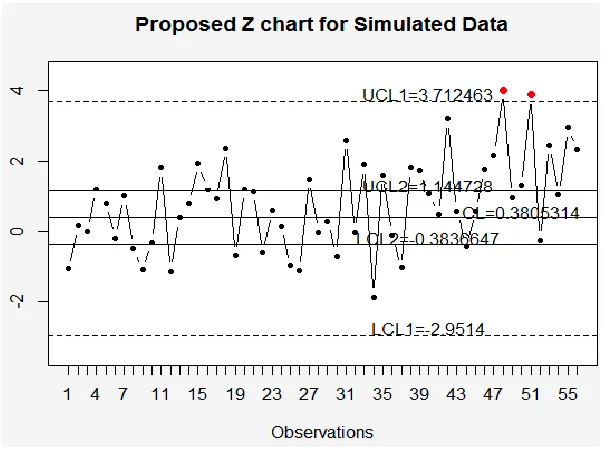
3.2. Simulated data
In this section, we compare proposed control chart with existing chart using simulated data. For this purpose, the first 28 observations are generated from two-piece normal distribution (TPN) with parameters μ=0, σ1=1 and σ2=1.5 (i.e. the in-control situation)
and the second set of the 28 observations from two-piece normal distribution with parameters μ=1.0, σ1=1 and σ2=1.5 (i.e. out-of-control situation having a shift of 𝛿
=1.0.To fix the ARL0 at 370, we have used k1=3.2587and k2=0.7474 for the proposed
process (with same shift as in proposed chart,𝛿 =1.0). Figure 4 shows the existing chart using single sampling.
Table 5: Comparison of ARLs when 𝒓𝟎 is 300 or 370.
𝛿
𝑟0= 300 𝑟0= 370
Proposed using Single sampling
k=3.0137
Proposed with k1=3.1740 k2=0.7856
Proposed using Single sampling
k=3.0891
Proposed with k1=3.2587 k2=0.7474
ARL1 ASS1 ARL1 ASS1 ARL1 ASS1 ARL1 ASS1
0.0 300.03 1.00 300.00 1.57 370.06 1.00 370.00 1.62
0.1 230.19 1.00 226.73 1.56 281.88 1.00 276.65 1.61
0.2 174.86 1.01 169.46 1.55 211.52 1.00 204.96 1.60
0.3 132.70 1.01 126.18 1.56 160.32 1.01 151.44 1.61
0.4 101.08 1.01 93.97 1.57 121.06 1.01 111.98 1.62
0.5 77.49 1.01 70.14 1.59 92.84 1.01 83.02 1.64
0.6 59.86 1.02 52.54 1.62 71.52 1.01 61.76 1.67
0.7 46.62 1.02 39.53 1.66 55.60 1.02 46.15 1.71
0.8 36.62 1.03 29.89 1.70 43.65 1.02 34.66 1.76
0.9 29.02 1.04 22.73 1.75 34.60 1.03 26.17 1.81
1.0 23.19 1.05 17.39 1.81 27.71 1.04 19.89 1.87
1.1 18.70 1.06 13.41 1.87 22.42 1.05 15.22 1.93
1.2 15.21 1.07 10.42 1.93 18.32 1.06 11.75 2.00
1.3 12.47 1.09 8.18 2.00 14.93 1.08 9.15 2.07
1.4 10.32 1.11 6.49 2.06 12.26 1.09 7.20 2.14
1.5 8.61 1.13 5.20 2.12 10.16 1.12 5.73 2.20
1.6 7.24 1.16 4.23 2.17 9.07 1.14 4.63 2.26
1.7 6.14 1.19 3.49 2.20 7.81 1.17 3.78 2.30
1.8 5.25 1.24 2.92 2.23 6.80 1.21 3.14 2.33
1.9 4.53 1.28 2.48 2.24 5.20 1.25 2.65 2.34
2.0 3.93 1.34 2.14 2.23 4.97 1.30 2.27 2.33
Figure 3. Proposed control chart for simulated data
Figure 4. Single sample control chart for simulated data
4. Concluding Remarks
Acknowledgements
The authors are deeply thankful to editor and reviewers for their valuable suggestions to improve the quality of this manuscript. This article was funded by the Deanship of Scientific Research (DSR) at King Abdulaziz University, Jeddah. The author, Muhammad Aslam, therefore, acknowledge with thanks DSR technical and financial support.
References
1. Santiago, E. and J. Smith. (2013) Control charts based on the exponential distribution: adapting runs rules for the t chart. Quality Engineering,. 25(2): p. 85-96.
2. Amin, R.W., M.R. Reynolds Jr, and B. Saad (1995) Nonparametric quality control charts based on the sign statistic. Communications in Statistics-Theory and Methods,. 24(6): p. 1597-1623.
3. Bai, D. and I. Choi (1995). (X) OVER-BAR-CONTROL AND R-CONTROL CHARTS FOR SKEWED POPULATIONS. Journal of Quality Technology, 27(2): p. 120-131.
4. Chang, Y.S. and D.S. Bai (2001) Control charts for positively‐skewed populations with weighted standard deviations. Quality and Reliability Engineering International,. 17(5): p. 397-406.
5. Al-Oraini, H.A. and M. Rahim (2002) Economic statistical design of X̄ control charts for systems with Gamma (< i> λ</i>, 2) in-control times. Computers & industrial engineering,. 43(3): p. 645-654.
6. Riaz, M., et al. (2014) On efficient phase II process monitoring charts. The International Journal of Advanced Manufacturing Technology,. 70(9-12): p. 2263-2274.
7. McCracken, A. and S. Chakraborti (2013) Control charts for joint monitoring of mean and variance: an overview. Quality Technology & Quantitative Management,. 10: p. 17-35.
8. Britton, E. and P. Fisher (1998) The Inflation Report projections: understanding the fan chart. Chart,. 8: p. 10.
9. Kimber, A. and C. Jeynes (1987) An application of the truncated two-piece normal distribution to the measurement of depths of arsenic implants in silicon. Applied statistics,: p. 352-357.
10. Simionescu, M., (2014) Fan chart or Monte Carlo simulations for assessing the uncertainty of inflation forecasts in Romania? Economic Research-Ekonomska Istraživanja,. 27(1): p. 629-644.
11. John, S., (1982) The three-parameter two-piece normal family of distributions and its fitting. Communications in Statistics-Theory and Methods,. 11(8): p. 879-885. 12. Figueiredo, F. and M.I. Gomes, (2013) The skew-normal distribution in SPC.
13. Aslam, M., et al., (2014) Designing of a new monitoring t-chart using repetitive sampling. Information sciences,. 269: p. 210-216.
14. Lee, H., et al., (2014) A control chart using an auxiliary variable and repetitive sampling for monitoring process mean. Journal of Statistical Computation and Simulation, (ahead-of-print): p. 1-8.
15. Banerjee, N. and A. Das, (2014) Fan chart: Methodology and its application to inflation forecasting in India. Departement of Economic and Policy Research, 16. Nadarajah, S. and S. Kotz, (2007) On the alternative to the Weibull function.