IMAGE DENOISING USING INDEPENDENT COMPONENT ANALYSIS
TECHNIQUE
Vishwajit K. Barbudhe, Assistant Professor
Jagadambha college of Engineering & Technology
Master of Engineering (ME), Electronics & Telecommunication Engineering Department, Yavatmal, India.
ABSTRACT
It is necessary to apply an efficient denoising technique to compensate for such data corruption. Image
denoising still remains a challenge for researchers because noise removal introduces artifacts and
causes blurring of the images. This paper describes different methodologies for noise reduction (or
denoising) giving an insight as to which algorithm should be used to find the most reliable estimate of
the original image data given its degraded version. Removing noise from the original signal is still a
challenging problem for researchers. There have been several published algorithms and each approach
has its assumptions, advantages, and limitations. This paper presents a review of some significant work
in the area of image denoising. After a brief introduction, some popular approaches are classified into
different groups and an overview of various algorithms and analysis is provided.
Keywords ( Image denoising , Independent component analysis technique )
Introduction
A quantitative measure of comparison is provided by the signal to noise ratio of the image. A very large
portion of digital image processing is devoted to image restoration. This includes research in algorithm
development and routine goal oriented image processing. Image restoration is the removal or reduction
of degradations that are Incurred while the image is being obtained. Degradation comes from blurring as
well as noise due to electronic and photometric sources. Blurring is a form of bandwidth reduction of the
image caused by the imperfect image formation process such as relative motion between the camera and
the original scene or by an optical system that is out of focus. When aerial photographs are produced for
remote sensing purposes, blurs are introduced by atmospheric turbulence, aberrations in the optical
recorded image is corrupted by noises too. A noise is introduced in the transmission medium due to a
noisy channel, errors during the measurement process and during quantization of the data for digital
storage. Each element in the imaging chain such as lenses, film, digitizer, etc. contribute to the
degradation.
Image denoising is often used in the field of photography or publishing where an image was
somehow degraded but needs to be improved before it can be printed. For this type of application we
need to know something about the degradation process in order to develop a model for it. When we have
a model for the degradation process, the inverse process can be applied to the image to restore it back to
the original form. This type of image restoration is often used in space exploration to help eliminate
artifacts generated by mechanical jitter in a spacecraft or to compensate for distortion in the optical
system of a telescope. Image denoising finds applications in fields such as astronomy where the
resolution limitations are severe, in medical imaging where the physical requirements for high quality
imaging are needed for analyzing images of unique events, and in forensic science where potentially
useful photographic evidence is sometimes of extremely bad quality. Let us now consider the
representation of a digital image. A 2-dimensional digital image can be represented as a 2-dimensional
array of data s(x,y), where (x,y) represent the pixel location. The pixel value corresponds to the
brightness of the image at location (x,y). Some of the most frequently used image types are binary,
gray-scale and color images. Binary images are the simplest type of images and can take only two discrete
values, black and white. Black is represented with the value „0‟ while white with „1‟. Note that a binary
image is generally created from a gray-scale image. A binary image finds applications in computer
vision areas where the general shape or outline information of the image is needed. They are also
referred to as 1 bit/pixel images. Gray-scale images are known as monochrome or one-color images. The
images used for experimentation purposes in this thesis are all gray-scale images. They contain no color
information. They represent the brightness of the image. This image contains 8 bits/pixel data, which
means it can have up to 256 (0-255) different brightness levels. A „0‟ represents black and „255‟ denotes
white. In between values from 1 to 254 represent the different gray levels. As they contain the intensity
information, they are also referred to as intensity images. Color images are considered as three band
information of the corresponding spectral band. Typical color images are red, green and blue images and
are also referred to as RGB images. This is a 24 bits/pixel image.
Literature survey on Principal Component Analysis
The two papers adopted different approaches, with the standard algebraic derivation given above being
close to that introduced by Hotelling (1933). Pearson (1901), on the other hand, was concerned with
finding lines and planes that best fit a set of points in p-dimensional space, and the geometric
optimization problems he considered also lead to PCs. In the 32 years between Pearson‟s and Hotelling‟s papers, very little relevant material seems to have been published, although Rao (1964)
indicates that Frisch (1929) adopted a similar approach to that of Pearson.
Literature survey on adaptive principal component analysis
One of the main difficulties in using principal component analysis (PCA) is the selection of the
number of principal components (PCs). There exist a plethora of methods to calculate the number of
PCs, but most of them use monotonically increasing or decreasing indices. Therefore, the decision to
choose the number of principal components is very subjective. In this paper, we present a method based
on the variance of the reconstruction error to select the number of PCs. This method demonstrates a
minimum over the number of PCs. Conditions are given under which this minimum corresponds to the
true number of PCs.
Ten other methods available in the signal processing and chemometrics literature are overviewed and
compared with the proposed method. Three data sets are used to test the different methods for selecting
the number of PCs: two of them are real process data and the other one is a batch reactor simulation.
Literature survey on Independent Component Analysis
The ICA algorithms above only consider the higher order statistics of the separate data maps recorded at
different time points, with no regard for the time order in which the maps occur. The so-called
„second-order blind identification‟ (SOBI) approach (Molgedey and Schuster, 1994) considers relationships
between multiple time points using an autoregressive model in which sources are assumed to have both
available Matlab (The Mathworks, Inc.) platform code for at least 22 methods of ICA decomposition
(Makeig and Delorme, 2004).
Algorithms and details on methods:-
Principal Component Analysis
The central idea of principal component analysis (PCA) is to reduce the dimensionality of a data set
consisting of a large number of interrelated variables, while retaining as much as possible of the
variation present in the data set. This is achieved by transforming to a new set of variables, the principal
components (PCs), which are uncorrelated, and which are ordered so that the first few retain most of the
variation present in all of the original variables.
Background Mathematics
Statistics
The entire subject of statistics deals with large dataset and its analysis in terms of the relationships
between the individual points in that dataset.
Standard Deviation
The Standard Deviation (SD) of a data set is a measure of how spread out the data is. The definition of
the SD is: “The average distance from the mean of the data set to a point”. The way to calculate it is to
compute the squares of the distance from each data point to the mean of the set, add them all up, divide
by (n-1) and take the positive square root. As a formula:
𝑠 = (𝑋𝑖− 𝑋 )
2 𝑛
𝑖=1
(𝑛 − 1)
Where s the usual symbol for standard deviation of a sample.
Variance
Variance is another measure of the spread of data in a data set. In fact it is almost identical to the
𝑠2= (𝑋𝑖− 𝑋 ) 2 𝑛
𝑖=1
(𝑛 − 1)
It can be noticed that this is simply the standard deviation squared, in both the symbol (s2) and the
formula (there is no square root in the formula for variance). s2 is the usual symbol for variance of a
sample. Both these measurements are measures of the spread of the data. Standard deviation is the most
common measure, but variance is also used.
Covariance
Standard deviation and variance only operate on 1 dimension, so that it could only calculate the standard
deviation for each dimension of the data set independently of the other dimensions. However, it is useful
to have a similar measure to find out how much the dimensions vary from the mean with respect to each
other.
Covariance is such a measure. Covariance is always measured between 2 dimensions. If you
calculate the covariance between one dimension and itself, you get the variance. If there was
3-dimensional data set (x, y, z), then you could measure the covariance between the x and y dimensions,
the x and z dimensions, and the y and z dimensions. Measuring the covariance between x and x, or y and
y, or z and z would give you the variance of the x, y and z dimensions respectively.
The formula for covariance is very similar to the formula for variance. The formula for variance
could also be written like this:
𝑣𝑎𝑟(𝑋) = 𝑋𝑖 − 𝑋 (𝑋𝑖 − 𝑋 )
𝑛 𝑖=1
(𝑛 − 1)
So given that knowledge, here is the formula for covariance:
𝑐𝑜𝑣(𝑋, 𝑌) = 𝑋𝑖− 𝑋 (𝑌𝑖− 𝑌 )
𝑛 𝑖=1
(𝑛 − 1)
Covariance is always measured between 2 classes. If we have dataset more than 2 dimensions, there is
more than one covariance that can be calculated. A useful way to get all the possible covariance values
between all the different dimensions is to calculate them all and put them in a matrix. So, the definition
for the covariance matrix for a set of data with n dimensions is:
𝐶𝑛×𝑛 = 𝑐𝑖,𝑗, 𝑐𝑖,𝑗 = 𝑐𝑜𝑣 𝐷𝑖𝑚𝑖, 𝐷𝑖𝑚𝑗 ,
where CnXn is a matrix with n rows and n columns, and Dimx is the x th dimension.
Matrix Algebra
This section serves to provide a background for the matrix algebra required in PCA.
(i). Eigenvectors : You can multiply two matrices together, provided they are compatible sizes. Eigenvectors are a special case of this. It is the nature of the transformation that the eigenvectors arise
from. Imagine a transformation matrix that, when multiplied on the left, reflected vectors in the line
y=x.
Then you can see that if there were a vector that lay on the line y=x, its reflection is itself. This vector
(and all multiples of it, because it wouldn‟t matter how long the vector was), would be an eigenvector of
that transformation matrix. What properties do these eigenvectors have? You should first know that
eigenvectors can only be found for square matrices. And, not every square matrix has eigenvectors.
And, given n X n matrix that does have eigenvectors, there are n of them. Given a 3 X 3 matrix, there are
3 eigenvectors.
Another property of eigenvectors is that even if you scale the vector by some amount before you
multiply it, you still get the same multiple of it as a result. This is because if you scale a vector by some
amount, all you are doing is making it longer, not changing its direction. Lastly, all the eigenvectors of a
matrix are perpendicular, i.e. at right angles to each other, no matter how many dimensions you have i.e.
orthogonal. This is important because it means that you can express the data in terms of these
Another important thing to know is that when mathematicians find eigenvectors, they like to find the
eigenvectors whose length is exactly one. This is because the length of a vector doesn‟t affect whether it‟s an eigenvector or not, whereas the direction does. So, in order to keep eigenvectors standard,
whenever we find an eigenvector we usually scale it to make it have a length of 1, so that all
eigenvectors have the same length.
(ii). Eigenvalues
Eigenvalues are closely related to eigenvectors. For each eigenvector, the corresponding eigenvalue is
the factor by which the eigenvector changes when multiplied by the matrix.
Calculations of Principal Components
The identification of subspace in which the data approximately lies will be calculated with the help of
Principal Components Analysis (PCA) tool.
Suppose we are given dataset x(i); i=1,...,m Lets x(i) for each i (n << m).
To develop the PCA algorithm, we need some preprocessing of data to normalize its mean and variance
as follows:
Suppose 𝑥1, 𝑥2, … , 𝑥𝑀 are Nx1 vectors
Step 1: Find mean 𝑥 = 1
𝑀 𝑥𝑖
𝑀 𝑖=1
Step 2: Subtract the mean: Φ𝑖 = 𝑥𝑖− 𝑥
Step 3: Form the matrix 𝐴 = [Φ1,Φ2,… ,Φ𝑀] (NxM matrix), then compute:
𝐶 = 1
𝑀 Φ𝑛Φ𝑛
𝑇 𝑀
𝑛=1
= 𝐴𝐴𝑇
(Sample Covariance matrix, NxN, characterizes the scatter of the data)
Step 5: Compute the eigenvectors of C: 𝑢1, 𝑢2, … , 𝑢𝑁
Since C is symmetric, 𝑢1, 𝑢2, … , 𝑢𝑁 form a basis,( i.e. any vector x ( or (𝑥 − 𝑥 ) can be written as a
linear combination of the eigenvectors): 𝑥 − 𝑥 = 𝑏1𝑢1 + 𝑏2𝑢2+ ⋯ + 𝑏𝑁𝑢𝑁 = 𝑁 𝑏𝑖𝑢𝑖
𝑖=1
Step 6: (dimensionality reduction step) Keep only the terms corresponding to the K largest eigenvalues:
𝑥 − 𝑥 = 𝐾𝑖 =1𝑏𝑖𝑢𝑖 where K<<N. The representation of (𝑥 − 𝑥 ) into the basis 𝑢1, 𝑢2, … , 𝑢𝑁 is
thus
𝑏1 𝑏2 … 𝑏𝐾
How to choose the principal components? To choose K, use the following criterion:
𝜆𝑖
𝐾 𝑖=1
𝑁𝑖=1𝜆𝑖 > 𝑇ℎ𝑟𝑒𝑠ℎ𝑜𝑙𝑑(𝑒. 𝑔. ,0.9 𝑜𝑟 0.95)
Geometrical Interpretation
1. PCA projects the data along the directions where the data varies the most.
2.These directions are determined by the eigenvectors of the covariance matrix corresponding to the
largest eigenvalues.
3.The magnitude of the eigenvalues corresponds to the variance of the data along the eigenvector
directions.
Properties and assumptions of PCA:- 1. The new variables (i.e., bi‟s) are uncorrelated.
2. The covariance of bi ‟s is: 𝑈𝑇𝐶𝑈 =
𝜆1 0 0
0 𝜆2 0
∙ ∙ ∙
∙ ∙ ∙
∙ ∙ ∙
0 0 𝜆𝐾
1. The covariance matrix represents only second order statistics among the vector values.
2. Since the new variables are linear combinations of the original variables, it is usually difficult to
interpret their meaning.
RESULTS
The Codes are written for PCA, Adaptive PCA, and ICA. These codes are simulated, synthesized and
implemented in Matlab. The results of simulation are reported here. The images which are obtained are
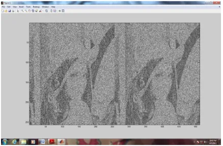
[image:9.612.194.421.388.528.2]as follows
Fig. Original image+ Noisy image
Matlab figure window shows original image in jpg format of 256 X 256 pixels with noisy image having
Gaussian noise with signal to noise ratio 6.816146 db, entropy 0.3334 , Variance 234.1728 , Correlation
0.882.
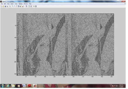
Fig. Noisy image + denoised image(JPG) by PCA
Matlab figure window shows original image in jpg format of 256 X 256 pixels with noisy image having
Gaussian noise with signal to noise ratio 7.379763 db, entropy 0.0244, variance 254.7538, correlation
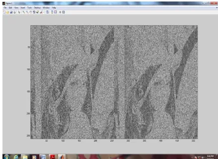
Fig Noisy image + denoised image(JPG) by Adaptive PCA
Matlab figure window shows original image in jpg format of 256 X 256 pixels with noisy image having
Gaussian noise with signal to noise ratio 6.936651 db, entropy 0.3216, variance 235.0867, correlation
0.0829.
Matlab figure window shows original image in jpg format of 256 X 256 pixels with noisy image having
Gaussian noise with signal to noise ratio 13.704733 db, entropy 0.2117, variance 243.1234, correlation
0.0488.
Fig. Noisy image + denoised image(JPG) by ICA
Matlab figure window shows original image in GIF format of 256 X 256 pixels with noisy image having Gaussian noise with signal to noise ratio 6.962064 db, entropy 0.3217, Variance 235.1129 ,
[image:10.612.198.417.422.566.2]Fig Noisy image + denoised image(GIF) by PCA
Matlab figure window shows original image in GIF format of 256 X 256 pixels with noisy image having
Gaussian noise with signal to noise ratio 8.099423 db, entropy 0.0237, Variance 254.7873 ,
Correlation0.0905 .
Fig Noisy image + denoised image(GIF) by Adaptive PCA
Matlab figure window shows original image in GIF format of 256 X 256 pixels with noisy image having
Gaussian noise with signal to noise ratio 13.751627 db, entropy 0.0415, Variance 243.1370, Correlation
0.2115.
Fig Noisy image + denoised image(BMP) by PCA
Matlab figure window shows original image in BMP format of 256 X 256 pixels with noisy image
having Gaussian noise with signal to noise ratio 6.967201 db, entropy 0.3210 , Variance 235.1199,
Correlation 0.0616 .
Fig Noisy image + denoised image(BMP) by Adaptive PCA
Matlab figure window shows original image in BMP format of 256 X 256 pixels with noisy image
having Gaussian noise with signal to noise ratio 7.809952 db, entropy 0.0238, Variance253.7528 ,
Correlation0.0906 .
Fig Noisy image + denoised image(BMP) by ICA
Matlab figure window shows original image in BMP format of 256 X 256 pixels with noisy image
having Gaussian noise with signal to noise ratio 13.699066 db, entropy 0.2115, Variance 243.1330,
CONCLUSION
The signal to noise ratio of an image under study is 8.5db. Principal component analysis will achieved
an improve value of signal to noise ratio as 8.69db. Adaptive PCA has proven to show an enhanced
value of signal to noise ratio upto 11.01db. Adaptive PCA has shown an improvement in noise
reduction. Furthermore with independent component analysis with local maxima algorithm we could
achieve an further enhancement value upto 15.18db of signal to noise ratio for the image under study.
For various type of image format we get the different signal to noise ratio, and by comparing the signal
to noise ratio and parameter table we can conclude that ICA is the best tool for the image denoising.
The improvement of signal to noise ratio proves that ICA is powerful tool for denoising of an image.
Some preliminary studies have been made about the effectiveness of Independent
Component Analysis. So we can conclude that ICA-based methods give, at least for their application,
significantly better results than PCA. The superiority of ICA over PCA is also implicit in the use of PCA
as a preprocessing step.
REFERENCES :
1) Ce Liu, Richard Szeliski, Sing Bing Kang And C. Lawrence, William T. Freeman,”Automatic Estimation And Removal Of Noise From A Single Image”, Ieee Transaction On Pattern Analysis And Machine Intelligence,Vol.30,No.2, February 2008 .
2) Potnis Anjali, Somkuwar Ajay And Sapre S. D.,”A Review On Natural Image Denoising Using Independent Component Analysis Technique” , Advances In Computational Research,Issn: 0975-3273,Volume 2,Issue 1,2010,Pp-06-14.
3) Xin Li And Michael T. Orchard,”Spatially Adaptive Image Denoising Under Over Complete Expansion”, 0-7803-6297-7/100, 2008 Ieee.
6) Nichol, J.E. And Vohra, V., Noise Over Water Surfaces In Landsat Tm Images, Hadamard Transform Spectral Imager. 2011 Cross Strait Quad-Regional Radio Science And Wireless Technology Conference International Journal Of Remote Sensing, Vol.25, No.11, 2004, Pp.2087 – 2093
7) James V. Stone,”Independent Component Analysis”, Volume 2, Pp. 907– 912,John Wiley & Sons, Ltd, Chichester, 2005
8) Qingming Qian , Bingliang Hu , Jun Xu , Caifang Liu , Xiaobing Tan ,“ A Novel De-Noising Method Based On Independent Component Analysis (Ica) For Dmd Based Hadamard Transform Spectral Imager, 2011 Cross Strait Quad-Regional Radio Science And Wireless Technology Conference