A NOVEL FILTER BASED PARTITIONING DECISION TREE MODEL FOR REAL TIME NETWORK SECURITY

(1)

ISSN: 1992-8645 www.jatit.org E-ISSN: 1817-3195

227

RECONSTRUCTION OF THE HUMAN RETINAL BLOOD

VESSELS BY FRACTAL INTERPOLATION

1

H. GUEDRI

,

2

J. MALEK,3H. BELMABROUK

1,2,3,

Faculty of Science Monastir, Tunisia

E-mail: [email protected], [email protected], [email protected]

ABSTRACT

This paper presents the fractal interpolation method of the human retina image. In the first part, we focus on the segmentation image with Skeletonization and identify different types of pixels. Secondly, using Douglas-Peucker algorithm to reduce the number of pixels in the image we try to keep a form close to the original. then, we used fractal interpolation( IFS ) to decompress the encoded image .To evaluate the image quality of the methodology using the peak signal-to-noise (PSNR).The results obtained show that the method of Douglas-Peucker reduces the size of the image from 92 to 96 percent and the PSNR values of fractal interpolation are between 27 and 36.9 db. We conclude with fractal interpolation can have a better quality image.

Keywords: Douglas-Peuker Algorithm, Fractal Interpolation, Retinal Blood Vessel Image.

1. INTRODUCTION

With the progress of information, it requires information storage and faster communication links. Store images in a reduced memory leads to a direct reduction in storage costs and faster data transmissions. These facts support the efforts of private companies and universities on new image compression algorithms. Images are stored on computers as collections of bits (a bit is a binary unit of information that can answer "1" or "0") representing pixels or dots forming the pixels.

The current standard method most popular compression relies on eliminating high frequency components of the signal by storing only the low frequency components (Discrete Cosine Transform Algorithm). We find this method used in JPEG (still images) [1] , MPEG (motion video), H.261 (video telephony on ISDN lines), and H.263 (video

telephony over PSTN lines) compression

algorithms [2].

Contrary for other conventional compression techniques, the fractal compression does not attempt conventionally compress byte composing the frame[3] [4]. The principle here is to replace the image with mathematical formulas [5] [6]. The fractal image compression has been proposed for the first time by Barnsley [3]. It shows that the fractal compression's policy that an image is a set of identical patterns in limited numbers [6] [7], to

which we apply geometric transformations

(rotations, symmetries, enlargements, and

reductions)[8] [9] [10]. This method, based on the theorem of collage, shows that it is possible to encode fractal images using transformations defining a few Contracting iterated function system (IFS) [11] [12] [13]. Barnsley proposed an algorithm to build, from a given image, a set of transformations the contracting representative [8] [9].

In the first part we looked skeletisation images of the retina, eventually, some behaviors of differentiation of the different classes of points: the end-points and the points of bifurcations (inner points, branches, cross over ...) [20] [21].In the second part, are interested in the Douglas Peucker algorithm to determine the characteristic points in the human retina image used [22] [23] [24]. Then in another section we present the theory of affine transformation for compression and decompression fractal [14] [15] [16]. The proposed method to estimate the decoded image quality is explained in the next section [25]. Finally, the last section presents some results.

2. ALGORITHM

(2)

[image:2.612.69.550.43.336.2]

228

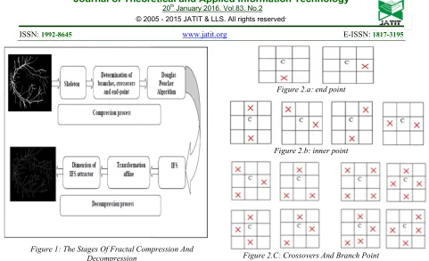
Figure 1: The Stages Of Fractal Compression And Decompression

3. IMAGE SEGMENTATION

2.1 Skeletonization of the human retina image

A real image is a very complex object to be manipulated without pretreatments. That is why it is often sought to simplify the information while retaining the most significant original image. A Skeletonization a binary image which corresponds to a kind of wire representation of the image elements, the aim is to represent a set with a minimum of information in a form that is both simple to extract and convenient to handle. It must account for geometrical properties and maintain relationships of connectivity: the same number of connected components, same number of holes each connected component which allows recovering the original shape [20] [21].

2.2 Detecting the endpoints and bifurcation

point from the image

The first step is to remove all of the coordinates of all the pixels containing information in the image. Then, for each pixel containing information, a mask is applied to determine the coordinates of the eight neighboring pixels [20] [21].

-

If only one neighbor pixel information so it is an end point (Figure 2.a).

-

If two neighboring pixels of the

information is such a developed interior (Figure 2.b).

[image:2.612.308.544.43.337.2]

-

If three or more adjacent pixels with information so it is a point of intersections and branch (Figure 1.c).

Figure 2.a: end point

[image:2.612.76.336.72.316.2]

Figure 2.b: inner point

Figure 2.C: Crossovers And Branch Point

4. DOUGLAS-PEUCKER ALGORITHM

[image:2.612.313.526.504.701.2]

This is a simplification algorithm of line. It retains the critical points that describe the overall shape of a line and removes all other points. The algorithm begins by connecting the ends of a line with a trend. The distance of each vertex relative to the trend line is measured perpendicularly. Closest to the line vertices those tolerances are eliminated. The line is then divided by the far top of the trend line, which has the effect of creating two trends. The remaining vertices are measured against these curves and ongoing process until all vertices within the tolerance range are eliminated (Figure 3) [22] [23] [24].

(3)

229

5. THE THEORETICAL BASIS

In this section we explain the theoretical basis of our model, starting by recalling some definitions in the IFS theory [8] [9] [10].

5.1 Iterated Function System (IFS)

An IFS (iterated function system) which when applied to a geometric object provides a fractal. These functions are affine and contracting. The term contractor means that when we apply these functions to a figure, the points of it but do not stray approach; there is no difference, a figure contained in a finite space is obtained. In the cases of dimension 2, the resulting image fractal therefore occupies a finished surface, which is none other than the surface of the initial object to a contour of infinite length. In this study we used, as contracting functions, affine transformations [13] [14] [15].

5.2 Affine transformation

An affine transformation is defined by a translation vector T and a transformation matrix V to obtain the coordinates of the point P' image of a point P in this transformation, applying the formula Vector:

OP ' = T.OP + V

If (x ', y') and (x, y) represent the coordinates of P 'and P, respectively, that can be translated by the following system of equations:

x' = ax + by + e (1)

y' = cx + dy + f

Where a, b, c and d are the coefficients of the matrix T and e and f are the components of the vector V [15] [16]. 5.3 Iterated function system (IFS) and fractal interpolation Let us represent the given set of data points as {(xn, yn) ЄIR2: n= 0, 1. . . N}. In general, the interpolation is applied to a subset of them, the interpolation points, represented as {(xi, yi) Є IR2: i = 0, 1. . . N}. the interpolation points partition the set of data points into interpolation intervals and may be chosen equidistantly or not. The greater the number of interpolation points the better the fit of the data, but more interpolation points result in a smaller compression ratio since more information is required to describe the interpolation function. The fractal interpolation iterative function system (IFS) is of the form {R2; Wn, n = 1, 2. . . N}, where, Wn have the following affine transformation structure: Let y axis has no rotation term, i.e. parameter b = 0 in formula (1). For every i = 1, 2. . . N. Solving the above equations results in: a (2)

c d ∗ (3)

e (4)

c d ∗ (5)

When 0 < di< 1, IFS has a single attractor and this attractor must be the diagram of certain continuous functions, and crossing original data point. Let the starting point be p0 = pi while [17] [18]. pi Є {p1, p2, . . . , pn}, the initial point can be selected at random, data series is x1< x2< x3 < …… < xn, start iteration operation from the initial point, use the initial point and any one group of affine functions to the generate the first point, then use the first point and any one group of affine function to generate the second point, continue to generate iteration point till the data point generated conforms to user demands.{Wn (P’n) = (x’n, y’n)| n=1, 2, 3. . . n’} is the fractal interpolation data point. Then N’ is the total number of interpolation data points [15] [19]. 5.4 Dimension of IFS attractor Fractal dimension (denoted by DF) in IFS is associated with the perpendicular scaling factor di. It can be learned from the theorem proposed in [2] [3]. that the total number of data points is n, ai ( i = 2,3,. . . ,n) follows the above-mentioned affine transformation IFS, when 0 <di< 1 and

∑

d

1

,suppose interpolation data points are not collinear, then attractor fractal dimension is the only real solution of the following equation [15][16]: ∑ d a 6

When x axis components of data points are equal-interval distributed, or xi – xi-1 = constant, then ai = 1/ (N - 1). Let perpendicular scaling component di = d be fixed. Then the equation above can be simplified as follows: d= (N-1) DF-2 (7)

6. PERFORMANCE EVALUATION

The PSNR computes the peak signal-to-noise ratio, in decibels, between two images. This ratio is used as a quality measurement between the original image and a compressed image.

(4)

230 squared error between the compressed and the original image, and the PSNR value represents a measure of the peak error [25].

For calculates the mean-squared error using the following equation:

MSE

!∗"

∑

‖f i, j

g i, j ‖

" ) * !

*

(8)

We confine our measurements to 1 bit per pixel binary images, so the peak signal-to-noise-ratio (PSNR) is computed as:

PSNR 10 ∗ log *

1∗23

456 9

f: represents the matrix data of our original

image

g: is the matrix of image data decompressed

m: represents the numbers of rows of pixels of

the images and i represents the index of that

row

n: represents the number of columns of pixels

of the image and j represents the index of that

column.

7. RESULTS

The skeleton reduces the number of image points worm a line while keeping its main aspect. It provides a simple and compact blood vessel of a shape that preserves many of the topological and size characteristics of the original shape. Thus, for instance, we can get a rough idea of the length of a shape by considering just the end points (and Figure 4.c) of the skeleton (Figure 4.b) and finding the maximally separated pair of end points on the skeleton. Similarly, we can distinguish many qualitatively different shapes from one another crossovers point (Figure 4.d). Figure 4.a shows one of the retinal images used from the STARE database[http://www.parl.clemson.edu/stare/probin g].

a

b

c

d

Figure 4.(A): Im0002.Jpg,(B): The Skeleton Of Im0002.Jpg,(C): Endpoint,(D): Crossovers Point

7.1 DP algorithm

[image:4.612.327.540.75.616.2] [image:4.612.82.305.525.710.2]

(5)

231 the execution of the algorithm DP the size of these information are reduced Figure 5.

ε =0.5 ε =0.8

ε =1 ε =1.3

ε =1.6 ε =2

Figure 5: Characteristics Points With Douglas-Peucker Algorithm

The Data Compression Ratio (DCR) is defined as follows: DCR= ((N−n)/N)*100%.

Table 1: Number of characteristics pixels and DCR% FOR different 8

9 2 1.6 1.3 1 0.8 0.5

n 237 263 292 340 401 545

n/N en % 3.11 3.45 3.8 4.4 5.2 7.1

Taux % 96.8 96.5 96.1 95 .4 94.7 92.8

The Douglas-Peucker algorithm reduce the amount of data storage, it constrict the number of points of a given line while keeping its main geometrical and topological properties. We see in TABLE1 that the compression ratio is about 92%, and it can be improved up to 96.6%, so the Douglas Peucker algorithm has a compression ratio high. It is noted that the compression ratio and the number of feature points vary according to the value of ε. if ε is high the number of items found is small and vice versa.

7.2 Simulation of the algorithm

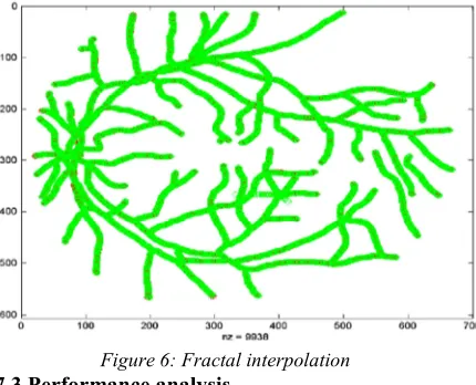
[image:5.612.316.531.292.466.2]

The following figure shows the simulation of the fractal interpolation to im0002.jpg image, we can say that are almost identical with the original image.

Figure 6: Fractal interpolation 7.3 Performance analysis

To assess the impact of fractal interpolation on image quality metrics used in this evaluation:

a. Calculates erroneous points

Table 2: Calculates erroneous points

fractal Dimension

1.541 1.645 1.747 1.857

Number of incorrect points

102 156 529 959

Number of the original points

7606 7606 7606 7606

(6)

232

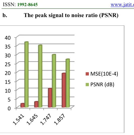
[image:6.612.86.313.74.303.2]

b. The peak signal to noise ratio (PSNR)

Figure 7.MSE And PSNR Values For Fractal Interpolation

Figure 7 gives the MSE values (8) and the values of PSNR (9) fractal interpolation for different values of the fractal dimension. We conclude that the values of PSNR are between 27 and 36.9 dB for the high value of the fractal dimension images, we have weak PSNR values (<30), therefore these images are of low quality. By against, for low values of their fractal dimension PSNR exceeds 30, as they are of acceptable quality images.

8. CONCLUSION

In this article, we studied the fractal interpolation of the image of the human retina. In the first part we interested in the image segmentation phase, we apply an image Skeletonization algorithm and determinate the different type of points (endpoint, bifurcation point, center line vessels). In the second part, using the Douglas-Peucker algorithm to determine the characteristic points from skeletons images, the algorithm advertised at a high compression rate can reach up to 96.6% .For the decompression phase us have used IFS fractal interpolation, the values of PSNR obtained between 27 and 36.9 dB in the high values of PSNR (PSNR> 30), the compressed images are acceptable quality images.To go further, we can go to the generation of blood vessels that are not included because of the limited resolution of the camera we use the L-system method

REFRENCES:

[1] M. I. Khalil, “Image Compression Using New Entropy Code”, International Journal of Computer Theory and Engineering, Vol. 2 No. 1 February, 2010; 1793-8201.

[2] K. H., Talukder and K. Harada, “Haar Wavelet Based Approach for Image Compression and Quality Assessment of Compressed Image”, IAENG International Journal of Applied Mathematics, 36:1, IJAM_36_1_9, 1 February 2007.

[3] M. F. Barnsley, “Fractals Everywhere”, Academic Press, Boston, 1988.

[4] B. B. Mandelbrot, “Fractals: Form, Chance and Dimension”, W.H. Freeman, San Francisco, 1977.

[5] K. Falconer, “Fractal Geometry, Mathematical Foundations and Applications”, John Wiley, Chichester, UK, 1990.

[6] H. M. Hastings and G. Sugihara, “Fractals: A User’s Guide for the Natural Sciences”, Oxford University Press, New York, 1993.

[7] J. Hutchinson, “Fractal and self-similarity”, Indiana Univ. Math. J., 30 (1981), pp. 713– 747.

[8] M. F. Barnsley, “Fractal functions and interpolations”, Constr. Approx., 2 (1986), pp. 303–329.

[9] M. F. Barnsley and L. P. Hurd,”Fractal Image Compression”, AK Peters, Wellesley, UK, 1992.

[10]D. S. Mazel and M. H. Hayes, “Using iterated function systems to model discrete sequences”, IEEE Trans. Signal Process, 40 (1992), pp. 1724–1734.

[11]P. R. Massopust, “Fractal Functions, Fractal Surfaces, and Wavelets”, Academic Press, SanDiego, 1994.

[12]Y. Zheng, “An Improved Fractal Image Compression Approach by Using Iterated Function System and Genetic Algorithm”, Computers and Mathematics with Applications 51 (2006) 1727-1740.

[13]T. Martyn, “A new approach to morphing 2D affine IFS fractal”, Computers & Graphics 28 (2004) 249-272.

[14]C. Chen, T. Lee, Y.M. Huang and F. Lai, “Extraction of characteristic points and fractal reconstruction for terrain profile data”, Chaos, Solitons and Fractals 39 (2009) 1732–1743. [15]R. Lopes, P. Dubois, I. Bhouri, H.

Akkari-Bettaieb, S. Maouche and N. Betrouni, “La géométrie fractale pour l’analyse de signaux médicaux : état de l’art Fractal geometry for

0 5 10 15 20 25 30 35 40

MSE(10E-4)

(7)

233 medical signal analysis: A review”, IRBM 31 (2010) 189–208.

[16]D. Vidya, R. Parthasarathy, T.C. Bina and N.G. Swaroopa, “Architecture for fractal image compression”, Journal of Systems Architecture 46 (2000) 1275-1291.

[17]S.K. Ghosh, Jayanta Mukherjee and P.P. Das, “Fractal image compression: a randomized approach”, Pattern Recognition Letters 25 (2004) 1013–1024.

[18]K. Igudesman, M. Davletbaev and G.

Shabernev."New Approach to Fractal

Approximation of Vector-Functions".Abstract and Applied Analysis, 8 February 2015. [19]F. Ling, Z. Wu, Y. Zhu, C. He and L. Zhu,

“Fractal approximation of the stress-strain curve of frozen soil”, Science in China Series D: Earth Sciences August 1999, Volume 42, Issue 1 Supplement, pp 17-22.

[20]Zhang, Y. Zhang and T. Zhang, “Automatic retinal image registration based on blood vessel feature point”, Proceedings of the First International Conference on Machine Learning and Cybernetics, Beijing, 4-5 November 2002.

[21]N. K. El Abbadi and E. H. El Saadi, “Automatic Detection of Vascular Bifurcations and Crossovers in Retinal Fundus Image”, IJCSI International Journal of Computer Science Issues, Vol. 10, Issue 6, No 1, November 2013.

[22]Douglas, D. H. and Peucker, T. K. (1973), “Algorithms for the reduction of the number of points required to represent a digitized line or its caricature”, The Canadian Cartographer, 10(2):112–122.

[23]Hershberger, J. & J. Snoeyink, “Speeding up the Douglas-Peucker line simplification algorithm”, In Proc. 5th Intl. Symp. Spatial Data Handling, 134-143. 1992.

[24]Ellen R. White, “Assessment of

Line-Generalization Algorithms Using

Characteristic Points”, The American

Cartographer Volume 12, Issue 1, 1985 [25]Q.Huynh-Thu, M. Ghanbari, “Scope of validity