Rapid Protoyping of a Single-Channel Electroencephalogram-Based Brain-Computer Interface

Abstract

ADCOCK, DAVID BROOKS. Rapid Prototyping of a Single-Channel Electroencephalogram-Based Brain-Computer Interface. (Under the direction of Edward Grant.)

This work describes the design, construction and implementation of a single-channel,

Rapid Prototyping of a Single-Channel Electroencephalogram-Based Brain-Computer Interface

by

D. Brooks Adcock

A thesis submitted to the Graduate Faculty of North Carolina State University

in partial fulfillment of the requirements for the degree of Masters of Science

Biomedical Engineering

North Carolina State University Raleigh NC, 27695

November 2006

approved by:

Lianne Cartee John Muth

Co-Chair of Advisory Committee

Dedication

Biography

Acknowledgments

I have been blessed by being surrounded by encouraging and supportive people. I would particularly like to thank. . .

•

My advisor, Dr. Edward Grant for allowing me to operate on the lunatic fringe. I still can’t believe

he let me do this project. No other advisor would have supported me this much in my eccentric research interests. For this I will always be grateful.

•

My committee, Dr Grant, Dr. Cartee and Dr. Muth. I did this project on a tight time frame and my

committee was generously accommodating and tolerant.

•

Nancy McKinney, Peggy Olive and Debra Paxton. These people went above and beyond to get

various documentation through at lightning speed. Without such diligent people I could not have finished. Thank you.

•

My subjects. These people sacrificed their time and a bit of hair to further my research. Thanks!

•

The CRIM team, Leo Mattos, Kyle Luthy, Carey Merritt, Meghan Hegarty, Matt Craver.

•

My family, my significant other, Liz, and the kittenz for their love.

•

My Mom for giving so much time to help me edit.

•

My Dad for being volunteering his time.

•

My biomedical role-models, Daniel Cline (EMT-P), Dr Brent Myers (MD) for teaching me the

Contents

List of Figures . . . viii

List of Tables. . . ix

Common BCI Abbreviations . . . x

1 Introduction . . . . 1

1.1 Motivation . . . 2

1.2 Project Goals . . . 3

1.3 Thesis Outline . . . 3

2 Review of Brain-Computer Interface Literature . . . . 5

2.1 Introduction . . . 5

2.2 Anatomical Disambiguation . . . 5

2.3 Signal Recording . . . 7

2.4 Feature Extraction . . . 7

2.5 Feature Analysis . . . 8

3 Exploited Principles of Neurobiology . . . 10

3.1 Introduction . . . 10

3.2 Indicators of Brain Activity . . . 10

3.2.1 Bioelectricity . . . 10

3.2.2 Hemodynamic Response . . . 12

3.3 Motor Pathways . . . 14

3.3.1 Prefrontal Cortex . . . 14

3.3.2 Posterior Parietal Cortex . . . 15

3.3.3 Premotor Area (PMA) and Supplementary Motor Area (SMA) . . . 15

3.3.4 Primary Motor Cortex (M1) . . . 15

3.3.5 Spinal Motor Pathways . . . 16

3.3.6 Application . . . 17

4 Design of a Custom Electroencephalogram Amplifier . . . 18

4.1 Introduction . . . 18

4.2 Electroencephalogram Design Goals . . . 19

4.3 Power Supply . . . 20

4.4 Stage 1: Pre-Amplifier . . . 21

4.5 Stage 2: Instrumentation Amplifier . . . 23

4.6 Stage 3: Band-Pass Filter . . . 23

4.7 Stage 4: Post-Amplification . . . 26

4.8 Additional Noise Reduction . . . 26

4.8.1 Overview . . . 26

4.8.2 Driven Right Leg . . . 26

4.8.3 Wire Braiding . . . 28

4.8.4 Printed Circuit Board Layout . . . 28

4.8.5 Faraday Cage . . . 28

4.8.6 Lead Selection . . . 29

4.8.7 Skin Preparation . . . 30

4.8.8 Software Filtering . . . 30

5.1 Introduction . . . 32

5.2 Electroencephalogram Data Acquisition . . . 33

5.3 Arm-Angle Data Acquisition . . . 34

6 Brain Computer Interface Software . . . 35

6.1 Introduction . . . 35

6.2 Design Goals . . . 36

6.3 Data Acquisition Procedure and Input Filtering . . . 38

6.3.1 Data Buffering and Display Threads . . . 38

6.3.2 Overlapped Band-Pass Filtering . . . 38

6.3.3 Arm Channel / Predicted Channel Acquisition . . . 41

6.4 Feature Extraction . . . 42

6.4.1 Component Wave Extraction . . . 42

6.4.2 Power Density and Autoregressive Coefficients . . . 42

6.5 Learning Paradigms . . . 46

6.5.1 Bayesian Networks . . . 46

6.5.2 Linear Discriminant Analysis . . . 46

6.5.3 Support Vector Machines . . . 47

6.5.4 Mutual Information . . . 47

6.5.5 Neural Networks . . . 48

6.6 Neural Network Architecture . . . 48

6.6.1 Input Size . . . 49

6.6.2 Hidden Layer Size . . . 49

6.6.3 Training Algorithm . . . 50

6.7 Output Smoothing . . . 51

7 Experiments and Results . . . 53

7.1 Introduction . . . 53

7.2 Experimental Setup and Procedure . . . 53

7.3 Subject Trials . . . 56

7.3.1 Subject 1 . . . 56

7.3.2 Subject 2 . . . 57

7.3.3 Subject 3 . . . 59

8 Conclusions . . . 63

8.1 Introduction . . . 63

8.1.1 System Safety . . . 63

8.1.2 Electroencephalogram Predictive Base . . . 63

8.1.3 System Cost . . . 63

8.1.4 Computer Platform . . . 64

8.1.5 Predictive Capacity . . . 65

8.1.6 Final Remarks . . . 65

8.2 Future Work . . . 65

8.2.1 Immediate Improvements . . . 66

8.2.2 Hardware Improvements . . . 66

8.2.3 Software Improvements . . . 66

8.2.4 Software Output . . . 67

8.2.5 Suggested Experiments . . . 67

List of Figures

1 Brodmann’s Areas . . . 6

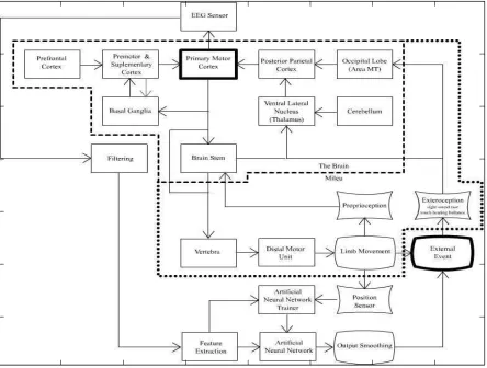
2 System Block Diagram . . . 9

3 Action Potential . . . 11

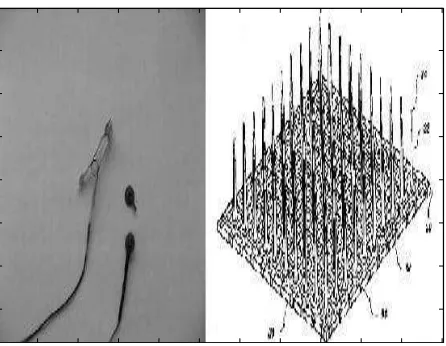
4 Invasive and Non-invasive EEG Sensors . . . 11

5 SQUID . . . 13

6 fMRI Image . . . 13

7 The Brain’s Motor Centers . . . 15

8 Homunculus . . . 16

9 EEG Brain Activation During Motor Movement . . . 17

10 International 10-20 EEG System . . . 18

11 Schematic: Power Supply and Layout . . . 21

12 Schematic: EEG Front-end Circuits . . . 22

13 Chebeshev and Butterworth Frequency Response . . . 24

14 Schematic: EEG Circuit . . . 25

15 Schematic: DRL Circuits . . . 27

16 60Hz Noise Rejection by DRL . . . 27

17 Example of Signal Aliasing . . . 32

18 Photo of Elbow Angle Sensor . . . 35

19 BCI Graphical User Interface . . . 37

20 Software Filter Error . . . 40

21 Recorded Alpha and Beta Waves . . . 42

22 Example of a Hilbert Transformation . . . 43

23 Power band trace computed from an EEG . . . 44

24 Instability of the Hilbert Transform . . . 45

25 Spectral Power Density Plot . . . 45

26 An Artificial Neural Network . . . 48

27 An Adaptive Filter Network . . . 49

28 A Neural Network Prediction of Arm Movement . . . 52

29 Output smoothing . . . 53

30 EEG Electrode Placement . . . 55

31 Subject 1: Graphical Results . . . 58

32 Subject 2: Graphical Results . . . 60

List of Tables

1 Abbreviations Used In This Paper . . . x

2 Filter PRO Specifications . . . 25

3 Neural Network Trials . . . 51

4 Vulnerable Populations . . . 54

5 Prohibited Medical Conditions . . . 54

6 A Neural Network training iteration performed on Subject 1’s data. . . 57

7 A Neural Network training iteration performed on Subject 2’s data. . . 59

8 A Neural Network training iteration performed on Subject 3’s data. . . 61

9 Expenses . . . 64

Common BCI Abbreviations

Table 1: Abbreviations Used In This Paper AC Alternating Current

AR Autoregressive

BCI Brain Computer Interface BMI Brain Machine Interface CMRR Common-Mode Rejection Ratio

DAQ Data Acquisition dB Decibel

DC Direct Current DRL Driven Right Leg EEG Electroencephalogram

EM Electromagnetic EOG Electroocculogram

FFT Fast Fourier Transform

fMRI Functional Magnetic Resonance Imaging GUI Graphical User Interface

ICA Independent Component Analysis IRB Institutional Review Board

LDA Linear Discriminant Analysis MEG Magnetoencephalogram

PCA Principle Component Analysis PET Positron Emission Tomography

1

Introduction

The defining characteristic of humankind has been its ability to evolve technologically as opposed to physically. Anthropologists state that as far back as seven million years ago, the ancestors of humans were creating primitive tools to extend their intrinsic ability [1]. Modern tools have gone so far as to allow us to rectify many of our own pathologies. Through technology, humans have all but absolved themselves from the Darwinian rat-race [2].

Despite the tremendous advances humans have made augmenting themselves, certain tech-nological borders have barely been breached. We adorn ourselves with various devices that allow us to accomplish remarkable things. However, few technologies have focused introspectively. The true goldmine of human technological evolution will be in intrinsic human enhancement. Ambulatory medi-cal devices that enhance or repair a human’s natural ability have barely been explored but offer great promise [2].

Pathology has driven research in intrinsic human improvement. The increased incidence of heart disease in the United States has motivated the development of artificial hearts and pacemakers that restore cardiac function [2]. The deaf and blind have recently experienced relief with implantable cochlear and retinal stimulators. Brain implants show promise for relieving central nervous system (CNS) deficits [2].

1.1

Motivation

Among the most exciting potential for human-augmenting technologies are enhancements to the human central nervous system (CNS). These technologies have the ability to enhance the lives of those with and without pathologies alike.

Traumatic and pathological injuries to the CNS create a sophisticated problem. Affronts to the CNS such as head trauma, spinal trauma, stroke, Parkinson’s disease, and Huntington’s disease usually result in irreparable damage [3, 4]. The human CNS, unlike the peripheral nervous system (PNS) does not readily repair itself. This implies that in order to fully recover from a severe CNS injury such as a stroke or spinal cord injury, artificial augmentation is needed. In the United States there is a large market for such augmenting devices [5]. According to the Spinal Cord Injury Information Network there are approximately 11,000 new spinal cord injuries (SCIs) each year [5]. This network claims that there may be 300,000 people in the United States alone currently living with some sort of SCI.

Augmentation of an injured CNS involves three steps. First, the CNS area that provides input to the injured area is identified and is used as input to the augmentation device. The processing for the injured area must be mimicked by the augmenting device. Finally, the effector that is controlled by the injured CNS area must be actuated. This actuation may involve replacing the end-effector or actuation device of the CNS or PNS beyond the site of injury [6].

The risks associated with direct neural interfacing are significant and thus make elective neural interfacing unattractive. However, a person with a pathology can afford to take greater medical risks, thus making such an interface a more attractive proposition. A person choosing to augment their CNS electively, would have to be assured that the procedure would be safe, which is now possible using several non-invasive interfacing procedures. These are an attractive option for the injured and uninjured alike [7].

electroen-cephalography (EEG). The application of this interface will lend mobility to someone who is completely or partially paralyzed. The system will be used in the rehabilitation of stroke or sports injury patients. Out-side of pathological augmentation, the system can be used to control an exoskeleton, allowing a person to lift multiple times their weight [8]. Although the potential applications are many, the primary goal of the research was to create a platform on which further research at the NCSU Center for Robotics and Intelligent Machines (CRIM) could be based.

1.2

Project Goals

The goal of this project was to create an EEG-based BCI platform for further research at the NCSU CRIM. The system was designed according to the following criteria.

1. The system must be non-invasive and safe for use by an untrained person.

2. The system must be scalp electroencephalogram based.

3. The system must be cost-effective.

4. The software must run on a standard PC.

5. The system must predict a one-degree-of-freedom kinematic variable from EEG activity alone.

1.3

Thesis Outline

Chapter 4 describes the design of the EEG used for acquiring brain signals. Motivation is pro-vided for the EEG design and its features are explored in signal order. Chapter 4 ends with a review of additional EEG signal processing tools for BCI applications.

Chapter 5 describes the methods used to acquire and store the recorded signals. EEG software is discussed in Chapter 6. Data gathering is described, followed by input filtering. Methods for computing neural synchronization are then explained. Finally, the learning algorithms considered for this project are explored.

2

Review of Brain-Computer Interface Literature

2.1

Introduction

Brain-computer interface (BCI) research is a permutation of functional neuroanatomy research [9–11]. The two fields are so closely related that they are often indistinguishable. As a general rule, studies of the applied use of neural activity can be categorized as BCI research. Studies that explore the temporal and spatial relationships between neural events and external events fall into the category of functional neuroanatomy [9, 12]. Many laboratories such as the McKeown laboratory and the Geor-gopoulos span both categories and are renowned by both the BCI and neuroanatomy communities [12]. In this chapter, categories of research are explored in signal pathway order. First, research in the identification of the spatial-temporal location of signals is discussed [12]. The preferences of various laboratories for recording these signals is then explored. Practices for extracting relevant data features from recorded signals are reviewed [13, 14]. Finally, studies using different feature analysis techniques are presented.

2.2

Anatomical Disambiguation

The first information that a BCI researcher needs to know is what spatial areas of the brain are responsible for the phenomenon under study. Korbinian Brodmann was one of the first people to make a scientific attempt to categorize the areas of the brain. He used tissue samples to segregate the brain into its distinct components. Brodmann’s areas, named for him, are now being confirmed to be of actual significance by more advanced scientific methods such as fMRI, PET, EEG and MEG. [12] Two of the biggest names in the field of anatomical disambiguation are Martin J. McKeown, M.D. and Apostolos P. Georgopoulos, M.D., Ph.D. Both researchers study the cortical activity associated with motor movement [9–11].

100

200

300

400

500

600

Figure 1: Brodmann’s Areas are groups of similar cells. These areas tend to be unique in function. (figure from [15])

[10, 11]. McKeown’s work has both proved the merit of ICA and demonstrated the coupling between the motor areas of the brain and body movements [10, 11].

Apostolos Georgopoulos [12] has gained widespread recognition for his analysis of cortical map-ping. He is reported to have demonstrated that neurons of the primary motor cortex (M1) encode for the force and direction of a limb. Further research in noninvasive recording techniques such as MEG has shown the efficacy of such methods for clinical use [9].

2.3

Signal Recording

The Nicolelis laboratory at Duke University is an excellent example of how a research center selects a recording technique and researches around that paradigm. The Nicolelis laboratory is known for its work in implantable electrodes in primates [13]. The technique around which their research is based involves implanting electrodes into the primary motor cortex and other supporting cortical areas [13, 18–20]. The Nicolelis laboratory has done quite a bit of work improving these electrodes [20], improving acquisition from these electrodes [18], as well as optimizing the algorithms used to make kinematic predictions of primate arm movement [13].

The Pfurtsheller laborotory from the University of Graz, Austria, has taken an alternative record-ing approach. Pfurtsheller has focused on improvrecord-ing non-invasive methods [21, 22]. The apparent goal of the Pfurtsheller laboratory has been to create a BCI that is available to the general public. Significant research has been put into making systems that do not require excessive biomedical equipment [14, 23]. Such non-invasive systems are extremely valuable.

2.4

Feature Extraction

Second in importance to knowing the spatial-temporal location of relevant brain signals, knowing the encoding scheme used by that specific area of the brain. For example, the light sensing retinal ganglia cells of the eye are excited by the absence rather than presence of light [12]. These encoding modalities dictate how the brain signal is extracted so that coherent information can be given to the feature analyzer. Two of the most common feature extraction techniques are the Hilbert transform and autore-gressive (AR) coefficients. Hilbert transformation provides the signal envelope and AR coefficients allow calculation of the band energy ratio. Papers from the Nicolelis and Pfurtsheller laboratories use both techniques [14, 19, 23, 24].

tech-niques for binary classification [25]. Sun supports spectral centroid as the superior method for binary classification [25].

2.5

Feature Analysis

100

200

300

400

500

600

3

Exploited Principles of Neurobiology

3.1

Introduction

Neuroscience studies of functional anatomy provide BCI researchers with the tools needed to in-terpret brain activity. There is a fine line between functional anatomy studies and BCI studies. Functional neuroscientists use medical imaging and learning algorithms to identify spatial-temporal brain patterns correlating to known external events. Alternatively, BCI researchers use medical imaging and learn-ing algorithms to interpret spatial-temporal brain patterns to drive external events. This chapter briefly discusses the neural anatomy and physiology that is interpreted by the BCI to drive external events.

3.2

Indicators of Brain Activity

3.2.1 Bioelectricity

The excitable cells of the body use electricity and ionic currents to transmit and store informa-tion. Excitable cells can be found all over the body including in brain, heart and muscle tissue. In the brain, neurons and glia are the primary excitable cells. Neurons are highly adaptive cells capable of learning. Glia are the cells that support neuronal activity. The electrical activity of neurons and glia can be measured as a means of interpreting brain activity. When neurons are at rest, they typically exhibit a resting electrical potential of around

−

70mV

[29]. When electrically excited, neurons permit ions to rapidly cross the cell wall [29]. The voltage level rises to a peak around

40mV

.

50

100

150

200

250

300

350

Figure 3: Electrical impulses generated by cells (action potentials) are the basis of nerve function. They can be recorded by brain interfaces to predict thought.

(figure from [30])

20

40

60

80

100

120

140

AP spikes are short lived and are thus less likely to overlap. In order to read the actual spike, nerve sleeve electrodes are needed [33]. Using these electrodes is highly invasive.

EEG is a popular method for BCI [14, 16, 17, 21, 23–28, 34, 35]. EEG has the advantage of having arbitrarily high temporal resolution. Spatial resolution can be theoretically increased to the single neuron level. Unfortunately in EEG, invasiveness accompanies spatial resolution. Electrodes placed in the brain can provide excellent data [13, 18–20]. Non-invasive scalp EEG signals provide only a rough view of the underlying neural activity. It has been said that interpreting scalp EEGs is like trying to listen into a single conversation in an sports stadium by sitting on the roof with a stethoscope.

Magnetoencephalography The orthogonal correlate to the electric field is the magnetic field. Move-ment of electrons or ions results in the creation of magnetic fields. In neuronal dendrites, ionic current flows are sufficient to create magnetic fields in the femtotesla range [36]. Magnetic fields are not dis-torted by cranial tissue as are electric fields [9]. MEG is superior to scalp EEG when evaluated on the basis of signal quality [9].

MEG was the initial, albeit short-lived, choice for brain signal acquisition. Initial research into scalp EEG quickly unveiled its shortcomings in spatial resolution. MEG offered better spatial resolution with temporal resolution equal to EEG. Georgopoulos’ paper on MEG interfacing made the choice look promising [9]. But, it was soon learned that MEG is prohibitively expensive. MEG acquisition requires the use of superconducting quantum interference devices (SQUIDs) to read the MEG signal. The further requirement of an electrically sterile aluminum and mu-metal enclosed room was also a deterrent to using MEG.

3.2.2 Hemodynamic Response

50

100

150

200

250

300

350

Figure 5: SQUID’s are sensitive magnetic field sensors used for MEG.(figure from [37])

20

40

60

80

100

120

140

160

180

200

Figure 6: fMRI can be used to acquire high spatial resolution, low temporal resolution brain activity maps. (figure from [40])

clinical medical diagnostics and functional neuroscience research, these tools can also be used for BCIs but are currently too unwieldy to be practical outside of a clinical environment [12, 38].

Positron Emitission Tomography An alternative to fMRI is positron emission tomography (PET). In PET, radioactive markers are injected into the blood supply. As the marker decays, positrons are emitted. Differential positron emission indicates the relative amount of blood located in a given area. PET is comparable to fMRI for BCI applications. PET trades magnetic field exposure for radioactive exposure. Where fMRI is simply not an option for subjects with ferrous metals in their body, PET can still be used.

EEG, MEG, fMRI and PET were all considered as potential means of brain monitoring for this project. The use of MEG, fMRI, or PET would have precluded making a portable, cost-effective system for use by future researchers in the CRIM laboratory. Scalp EEG, although lacking in spatial resolution, meets all the design criteria this project. Should higher spatial resolution be needed for future work, MEG, fMRI, PET, or invasive EEG might be used.

3.3

Motor Pathways

Brain-computer interfaces emulate the natural motor pathways of the central nervous system. A complete understanding of the functional anatomy of the motor pathways is required for creating a functional BCI. Studies using fMRI, PET and implanted electrodes reveal that certain brain areas can be used to predict motor movements [9, 12, 13]. The raw data is typically analyzed with statistical methods such as principle component analysis (PCA), independent component analysis (ICA) or linear discrimi-nant analysis (LDA) to reveal how strongly each area of the brain correlates to motor activity [16, 34, 41]. It is consistently demonstrated that despite individual variations amongst subjects, specific brain areas are related to certain functions.

3.3.1 Prefrontal Cortex

50

100

150

200

Figure 7: The brain’s motor areas connect to allow coordinated movement. (figure contains copyrighted material from [42])

3.3.2 Posterior Parietal Cortex

The posterior parietal cortex (PPC) provides the motor areas of the brain with the environmental information needed to formulate motor movements. The PPC consists of two areas, Brodmann’s area 5 and area 7. Brodmann’s Area 5 of the PPC receives information from the primary sensory cortex (S1) relating current body position and tactile information. Brodmann’s Area 7 of the PPC receives visual feedback from the occipital lobe. See Figure 1. [12]

3.3.3 Premotor Area (PMA) and Supplementary Motor Area (SMA)

The PMA and SMA (Brodmann’s Area 6) deal with motor planning. Studies with monkeys show that intended movements are queued in these areas here until they are executed. Artificial electrical stimulation of these areas results in complex motor movements. The PMA and SMA take inputs from the basal ganglia. The PMA feeds to the reticulospinal motor neurons which synapse with proximal motor units. The SMA feeds directly to distal motor units. [12]

3.3.4 Primary Motor Cortex (M1)

50

100

150

200

Figure 8: The Homunculus represents what a human would look like if each body part was proportional to the size of the brain area responsible for its control.

(figures contain copyrighted material from [42, 43])

Layer V pyramidal neurons (Betz cells) are the primary transmitters of motor commands to lower motor neurons from M1. Inputs to Betz cells are from other cortical areas such as the PMA and SMA. Inputs also come from the cerebellum and pons via the ventral lateral nucleus of the thalamus. The most recent thoughts about Betz cells are that they encode for the force and direction of motor movements. This implies that decoding to specific motor units is done at the level of the brain stem or spinal cord. [12]

It is also of note that M1 adheres to a consistent cortical mapping among species. The human M1 is consistently mapped according to the “homunculus” [12]. Artificial stimulation of a given location area mapped by the homunculus results in a motor movement of that area. This consistency can be employed to the advantage of the BCI researcher.

3.3.5 Spinal Motor Pathways

50

100

150

200

Figure 9: EEG recordings of brain activity during left- and right-sided motor movements. (figure from [35])

pathways synapse with lower motor neurons.

3.3.6 Application

It is consistently shown that M1 provides the best predictor of motor movement [16]. Other areas such as the PMA and SMA can enhance predictive abilities of a system when used in conjunction with M1 [13]. Nicolelis places implantable electrodes in M1, the PMA and other locations to improve predictive quality [13]. The disadvantages of using locations other than M1 are that the encoding of the motor movement becomes increasingly abstract. The least abstract reading would be at the level of motor unit nerves themselves, but this would no longer be a brain interface but more like an electromyogram interface.

50

100

150

200

Figure 10: The International 10-20 EEG System is a method of EEG lead placement.

4

Design of A Custom Electroencephalogram Amplifier

4.1

Introduction

Integral to the BCI system is how brain activity is measured. The human central nervous system is an orchestra of interconnected neurons, glia, and support tissue that broadcast multiple indicators of mental activity. A spectrum of tools exists for measuring these indicators ranging from bulky, costly but accurate fMRI, to the portable, inexpensive, and inaccurate scalp EEG. All of these tools create a window into the mind of a test subject [12], yet none of the tools serves as a ubiquitous interface for all BCI applications. PET and fMRI, for example, both provide a moderate-to-high resolution, real-time view of brain activity, but neither is portable enough to be used outside of a clinical environment. Scalp EEGs are highly portable but are capable only of detecting gross brain activity. This inadequacy may be overcome by replacing scalp EEG with scalp MEG.

is highly effective but precludes use by the general population. Furthermore, communication from a brain implant is limited to the area in which it is implanted. More often than not, signals from multiple areas of the brain are desirable. The Nicolelis laboratory deliberately targets carefully chosen brain areas; a general BCI user may require a more adaptable solution [13]. The research of Pfurtscheller et al., reinforces the merit of an adaptable system. Pfurtscheller et al. cite their work showing that multiple-lead, subject-customizable, EEG-based BCIs achieve higher accuracy than single-lead EEG-based BCIs [24].

In order to be practically applicable, a BCI system must not be overly expensive, bulky, invasive, or specialized. These constraints are in direct opposition to recording quality, which is also critical for a functional BCI application. Until technologies such as fMRI and MEG become more portable and affordable, the only brain-interface solution that has any practical application for applied BCI is scalp EEG. At roughly 2000 US dollars per system, EEGs are the cheapest solution but are hardly a bargain. EEG experts such as Stephen Luck assert that even with a top-of-the-line system, experiments must be performed in an electrically sterile environment [44]. Such requirements are impractical for most non-clinical BCI applications.

The need for a low-cost, highly-portable, noise-impervious EEG system motivates the need to construct a custom EEG amplifier. The advantages of a custom EEG amplifier are numerous. Organiza-tions such as OpenEEG have shown that a custom EEG amplifier can be built for around 200 US dollars. Basic biosignal amplifiers such as EEG amplifiers are not large circuits and can be custom designed to be highly portable. Furthermore, custom filters can be implemented to attack noise bands. A properly designed EEG amplifier could be highly effective for multiple BCI applications.

4.2

Electroencephalogram Design Goals

Hence, the goal of this phase of the project is to create a general-purpose EEG amplifier with the follow-ing features...

•

Maximum safety

•

Minimal cost

•

Maximum noise rejection

•

Driven-right-leg active noise cancellation

•

Strict band-pass filtering between 0.1Hz and 40Hz

•

Maximum portability

•

Battery powered

•

Single-channel differential analog input

•

Multiple analog outputs with varying net gains

4.3

Power Supply

Power for the EEG amplifier comes from an isolated

±

6V

dc supply.

18V

dc is supplied by two

series 9-Volt batteries. Two

6V

dcvoltage regulators (78x06) are cascaded to produce

+

0V

dc,

+

6V

dcand

+

12V

dc voltage outputs relative to battery ground. The

+

6V

dcterminal is selected to be

Ground

analog.

The other two outputs thus become

+

6V

dcand

−

6V

dcrelative to

Ground

analog.

The battery driven

±

6V

dc voltage configuration provides superior safety, noise rejection and

50

100

150

200

250

300

350

400

Figure 11: Schematic of the EEG power supply circuit and circuit layout.

Although battery-driven circuits have less intrinsic noise than outlet voltage sources, they are not immune to noise. Natural fluctuations in circuit power consumption result in power voltage fluctuations as voltage regulators adapt to increased power demands. Power voltage fluctuations can be translated to recorded signals via fluctuating amplifier gains. Placing capacitance between the leads of the power supply provides temporary power sources that can respond instantly to fluctuating power demands [45]. These capacitors stabilize the power supply, thus preventing power supply noise from being translated to the signal.

In the PCB layout, power supply traces are routed as far as possible from signal traces in order to prevent EM crosstalk between power and signal. The

Ground

analog node is expanded into a large

plane, filling in gaps between signal traces. This technique grounds external EM interference that would otherwise be induced between signal traces. These noise reduction techniques further stabilize the signal [45].

4.4

Stage 1: Pre-Amplifier

50

100

150

200

250

300

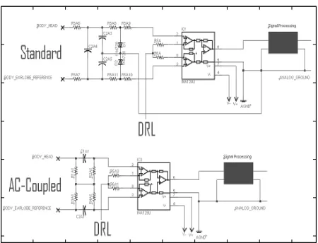
Figure 12: Comparison of AC-Coupled and non-AC-coupled front-ends for biosignal amplifiers

clipped resulting in the addition high-frequency components. Bioelectric signals such as EEG and EKG are extremely small

10µV

to

100mV

. They can be amplified at high gains without risking saturation.

Two common noise signals can be expected on the input lines along with the desired bioelectric signal: high voltage transients and 60Hz noise. High voltage transients are large, slow changes in skin surface potential caused by the accumulation of various types of charge. 60Hz noise is a byproduct of EM coupling between wires in a circuit and the power wires that are abundant in buildings. Other EM spectra are also picked up on wires, however they are far less powerful than 60Hz interference. The general term for such signals is common-mode noise because the interference is imparted equally on all leads. Voltage transients and common-mode noise are both often more pronounced than the desired signal to be read [46]. These noise sources can thus pose a saturation risk [46] for the differential op-amp.

An improved front end eliminates the bias path to ground by creating a reverse bias path. This modification was confirmed experimentally to increase noise rejection greatly.

4.5

Stage 2: Instrumentation Amplifier

The first amplification stage is an INA129U surface-mount, differential, instrumentation amplifier. Like most differential op-amps, the CMRR of the INA129U increases with gain [47, 48].

Table: from INA129 data sheet showing CMRR as a function of Gain

The highest gain possible is selected for the first amplification stage to maximize CMRR. Blocking noise in this way, before it cascades to later stages, means that the noise will not have to be removed later. Gain is set by two equal gain resistors according to the equation

G

=

1

+

4.94kΩ

Rgain [47].

56

Ω

Gain resistors are used to set a gain of approximately 100. This results in a CMRR of approximately 125 dB [47]. This amplification is the highest achievable without risking amplifier saturation.

Although the INA129 is available in both PCB surface-mount (SO8) and through-hole (DIP8) packages, surface-mount is preferable for low noise applications [45].

4.6

Stage 3: Band-Pass Filter

The signal passed from the initial amplification stage is a composite of EEG, motion artifact, and electrical interference. The amplitude of the EEG, although significantly amplified, is still only in the single millivolt range. This small EEG signal lies on the spectrum of about 1Hz to 35Hz [27, 49]. Analysis of the signal spectrum at this stage reveals a broad spectrum including a large spike at around 60Hz. This spike is the residual after common-mode noise rejection.

20

40

60

80

100

120

140

160

180

200

220

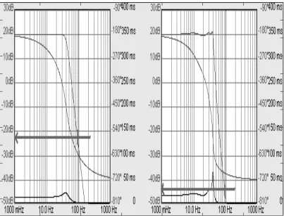
Figure 13: Chebyshev have better greater attenuation 68dB) at 100Hz than do Butterworth filters (-47dB) for the same order and cutoff frequency

the sampling frequency to be culled to make aliasing negligible. The sampling frequency is commonly referred to as

f

s. Half the sampling frequency is commonly referred to as the Nyquist frequency, or

f

N.

Many biosignal amplifiers employ first- or second-order Butterworth filters to prepare the signal for sampling because Butterworth filters are maximally flat in their pass band. An alternative to a Butter-worth filter is a Chebyshev filter which is not maximally flat in its pass-band. Unfortunately, Chebyshev filters exhibit ripple in the areas immediately around the cutoff frequency. To their advantage, Chebyshev filters exhibit a far steeper cutoff than Butterworth filters of the same order. Butterworth filters exhibit a gradual roll-off.

The filtering specifications of this device call for strict filtering between 0.1 and 40Hz. It is desired to have 60Hz frequencies attenuated by a minimum of 20dB to avoid 60Hz saturation of the amplifier. Signals above

f

N need to be attenuated so drastically that they can be negated. 20dB attenuation is

if frequency components above

f

Nwere large enough to be sampled.

The overall band-pass filter used here is a combination of a 6th-order, low-pass active Cheby-shev filter and a passive AC-couple (a capacitor in series). Sixth-order filters are absurdly difficult to design by hand. If a circuit is designed correctly, and the transfer function is computed correctly (both of which are unlikely), components must still be selected to achieve the desired filtering characteris-tics. Furthermore, component values must be commercially available. Fortunately, Texas Instruments has designed a powerful and free software package called “Filter Pro” that designs filters given desired parameters passed to the function. This program was used and given the following constraints.

Table 2: Specifications given to Texas Instruments’ Filter PRO software for the design of the EEG filter. Cutoff Frequency 40Hz

Filter Type Chebyshev Order 6

Configuration Multiple Feedback (MFB) Fully Differential NO

Resistor Series E12 Capacitor Series E6

Gain A 10 Gain B 1 Gain C 1

From the constraints issued to Filter Pro the following filter was designed. When prototyped, the circuit exhibited nearly identical behavior to the Filter Pro prediction. An AC-couple was selected by experimentation. The filter was attached to a spectrum analyzer and a range of AC-couple capacitors were tried until one yielded the desired outcome. Initial designs included an active high-pass filter. It was found on the spectrum analyzer that better performance was obtained by a simple AC-couple.

4.7

Stage 4: Post-Amplification

50

100

150

200

250

300

350

400

450

Figure 14: Complete schematic of the EEG circuit.

This is sufficient for ECG, however, EEG requires further amplification by 10 to 100. Such amplification results in an EEG signal with a peak-to-peak voltage of about 2 volts.

The amplifier designed in this project amplifies the signal in this stage by a factor of 10. Output is routed to an output pin. The input to this amplification stage is also routed to a second output pin so that the signal can be analyzed before amplification.

4.8

Additional Noise Reduction

4.8.1 Overview

Even with the construction of a low-noise EEG circuit, many factors can still contribute to noise. EM detection on wires, skin impedance, motion artifact, and PCB noise all degrade signal quality. This section describes techniques to overcome these obstacles to signal integrity.

4.8.2 Driven Right Leg (DRL)

50

100

150

200

250

300

350

400

Figure 15: Examples of DRL circuits. Top: standard DRL, Middle: integrating DRL. Bottom: transcon-ductance DRL.

sources were found that thoroughly describe their design criteria.

The general principal of the DRL circuit is to read the common-mode noise signal from between the

R

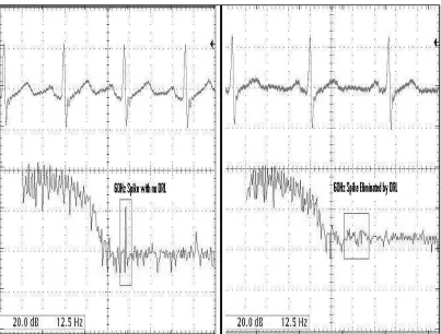
gainresistors of the differential instrumentation amplifier. This signal is buffered and added to noise

signals from other leads. The signal is then fed back into the body via an amplifier. Experiments showed that Webster’s design has superior noise rejection quality. Signal spectral analysis revealed that the act of attaching the DRL electrode to the body virtually eliminates 60Hz noise instantaneously.

For its superior performance, Websters DRL design was implemented to improve the CMRR.

4.8.3 Wire Braiding

50

100

150

200

250

300

350

400

Figure 16: Attaching a DRL circuit eliminates the 60Hz spike in the biosignal trace.

4.8.4 Printed Circuit Board Layout

Circuit layouts have many problems caused by flat traces in close proximity exhibiting mutual capacitance. Traces that are separated by some distance may also transduce EM flux. Carter describes many circuit layout techniques for the minimization of noise artifact [45]. Techniques used in the EEG PCB layout are listed below.

•

Traces are orthogonal wherever possible

•

The ground plane is large in order to sink, distribute, and negate interference

•

Power supply circuitry is as far as possible from signal circuitry

•

Signal circuitry is as close together as possible to eliminate distance losses and EM pickup (short

•

No digital circuitry was placed on the board, reducing high-frequency interference from digital

switching

4.8.5 Faraday Cage

A Faraday cage was built into a plastic carrying case. Fine wire-mesh copper screen was used to line the entire inside of the box. The box is groundable through a connection tab on the box’s exterior. Experiments showed that this box is highly effective at reducing external EM interference. An experiment was performed where all leads were disconnected from a subject, thus receiving maximum EM interfer-ence. EM noise was analyzed under different shielding conditions. The circuit and leads were placed in the grounded cage and the lid slowly closed. As the box was closed, EM was rejected. The Faraday cage is a barrier to outside noise. This cage is not particularly useful because the leads, the primary receptors of interference, must remain outside the box. For this reason the cage was abandoned for the final design.

4.8.6 Lead Selection

Much experimentation was done with leads. Initial attempts to make leads were unsuccessful. Webster’s Medical instrumentation illuminates part of the problem. The electrode at the skin interface must be made of specialized conductors. Leads must interface with the skin using certain types of metals that exchange ions for electrons. Silver chloride (AgCl), for example, emits an electron in response to a cation. Conversely, it emits a chloride ion when stimulated by an electron.

Ag

⇋

Ag

+

+

e

− (4.1)

Ag

+

+

Cl

−

⇋

AgCl

↓

(4.2)

performance. Inexpensive, alligator clips yield the second best performance but are prone to noise. Custom leads are so prone to noise that a usable signal cannot obtained. Shielded leads perform better than unshielded leads. Unfortunately, commercial shielded leads were too expensive for this design iteration.

4.8.7 Skin Preparation

Skin surface impedance has a tremendous effect on signal quality [51]. Mismatched impedance causes differential electrical transduction between the leads, which translates directly to the voltage mea-sured by the differential amplifier [49]. There are several methods for overcoming this, the simplest of which is to prepare the skin with a commercial electrode preparation gel. NuPrepTMis a slightly abrasive sterilizing gel that is applied to a cotton swab and rubbed over the desired electrode area. This action gently removes the top layer of dead skin and cleans the electrode site. After preparation, the electrodes have an equal, low impedance connection site on the skin.

4.8.8 Software Filtering

Noise can also be subtracted in software. Simple discrete-time Fourier-transform-based filtering can be employed to control selected bands. More complex filtering methods are suggested by Clancy, Hamilton, Erfanian, LevKov and Osdamar [52–56].

These methods of software filtering apply advanced spectral analysis to selectively remove arti-fact signals such as electroocculogram (EOG) and motion artiarti-fact. With the exception of Levkov’s subtrac-tion procedure, none of these systems were implemented because of limited computasubtrac-tional resources.

tracting RG from SG. Multiple leads are required to perform a subtraction procedure, therefore Levkov’s methods were not implemented in the final design. Single-lead noise-rejection methods were implented.

SG

=

V

signal to ground

+

Noise

common−mode (4.3)

RG

=

V

re f erence to ground

+

Noise

common−mode (4.4)

SR

= (

V

signal to ground

+

Noise

common−mode

)

−

(

V

re f erence to ground

+

Noise

common−mode

)

(4.5)

=

V

signal to ground

−

V

re f erence to ground (4.6)

50

100

150

200

250

300

350

400

Figure 17: Example of Signal Aliasing.

5

Data Acquisition

5.1

Introduction

Analog data must be acquired by a computer in order to do the processing needed for a BCI. The goal of this BCI was to predict arm-angle based on EEG activity from a single head lead. Both arm-angle and EEG activity are acquired by a National Instruments PCI-6025E DAQ. EEG activity and arm angle are converted to analog electrical signals that are sampled by the DAQ at 300Hz.

The sampling frequency,

f

s, of 300Hz is based on the Nyquist criteria of data sampling. This

criteria states that the lowest frequency at which a signal may be sampled is the Nyquist frequency. The Nyquist frequency is equal to half the sampling frequency. If the greatest frequency component of a sampled signal exceeds this frequency, aliasing will occur.

capability. Most BCI applications report sampling frequencies of around 120Hz [27]. This is inadequate for this application because it is below the Nyquist frequency. Sampling at an arbitrarily chosen rate of 1.5 times the Nyquist frequency, 300Hz, results in better accuracy than sampling at the minimum Nyquist frequency. Sampling at 300Hz also results in data sets of manageable size.

Calculating the data acquisition rate reveals that data management is quite feasible. Sampling at 300Hz results in 18000 samples per minute, per channel. At 12-bit sampling resolution, this equates to 216000 bits (27000 bytes or about 26.4kBytes) per minute, per channel. As two channels (EEG and arm angle) are being sampled, a total of 52.7kB are being sampled per minute. At this rate it would take 19.4 minutes to accrue 1MB of data. This data size is manageable considering that only ten minutes of data samples are required to train a BCI [16]. Most personal computers now have up to 2048MB (2GB) or more RAM. Were RAM to be used strictly for data storage, a personal computer with 2GB of ram could store 27.6 days worth of data. This indicates that the data requirements of this BCI are well within the processing power of even a modest home PC.

5.2

Electroencephalogram Data Acquisition

The EEG signal begins as a bioelectric signal produced by groups of neurons in the brain. The signal causes ions to move locally within tissue. These ions instigate a chemical reaction in the silver chloride (AgCl) EEG electrodes. This chemical reaction results in the emission or absorption of electrons. Electrons flow preferentially along copper lead wires to a differential op-amp where they are transduced into a powered electrical signal. This signal is amplified, filtered in hardware, amplified again, and trans-mitted as a large analog voltage to a data acquisition device. Low noise data acquisition is made possible by separating the digital sampling circuitry of the DAQ from the sensitive analog circuitry of the EEG sen-sor. To further make the EEG signal as noise free as possible, the EEG channel on the DAQ is connected physically as far apart from the arm DAQ channel as possible to prevent electrical crosstalk.

rails this equates to a voltage sensitivity of about

3mV

. This sensitivity is sufficient for reading the small EEG waves which are amplified to a peak to peak amplitude of around

20

−

30mV

. Larger EEG waves have peak-to-peak amplitudes of

200

−

300mV

. Voltage transients have amplitudes in the volt range. These EEG signals are sampled, buffered on the DAQ, and read into Mathworks Matlab7.1TMfor processing and permanent storage.

5.3

Arm-Angle Data Acquisition

The position of the human elbow is regulated by local lower motor neurons and upper motor neuron inhibition of the lower motor neurons. Elbow activity is cortically controlled by the activation of upper motor neurons inhibiting muscular opposition to the activity. In other words, flexion is controlled by the inhibition of extension-lower-motor neurons and extension is controlled by the inhibition of flexion-lower-motor neurons. [12]

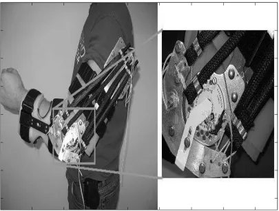
Indirectly, elbow angle indicates the relative activity of the upper motor neurons controlling the elbow. For this BCI, a special elbow brace, originally designed by NCSU graduate student Carey Merritt, was modified to sense elbow angle [57]. This was achieved by the addition of a potentiometer sensor to the elbow brace that changes resistance as a function of brace angle.

50

100

150

200

250

300

350

Figure 18: Elbow angle sensor.

6

Brain Computer Interface Software

6.1

Introduction

All the processing of the BCI is done in software in real-time. The BCI hardware is responsible for providing the software with clean, meaningful data. Software then performs all of the signal processing necessary to predict actual arm movement in real-time based on the EEG signal. Signal filtering, alpha-and beta-wave extraction, power-balpha-and analysis, alpha-and neural network arm-angle-prediction are performed in real-time. Neural network training is performed off-line.

discretion and convenience.

The program was developed in Mathworks Matlab7.1TM. Of the available environments in which a signal analysis platform could be built, Matlab provided the most efficient environment for rapid pro-totyping and development. Matlab Signal Processing, Data Acquisition and Neural Network toolboxes were used.

The tools built into Matlab allowed rapid iterative development. Signal processing requires many complex algorithms such as the fast-Fourier-transform frequency-analysis method and Levenberg-Marquardt neural-network-training method. Matlab has many such methods already built-in and opti-mized. A significant part of the software design time involved experimenting with different algorithms for signal analysis. Use of Matlab enabled the rapid development of a functional system. See Figure 2.

6.2

Design Goals

The purpose of the software was to provide an arm-angle prediction based on analog EEG data. The software was supplied with the analog EEG signal via a data acquisition device. Actual arm angle was also supplied via the data acquisition device for evaluation of accuracy. The actual arm angle was used to train the learning algorithm. The actual arm angle was NOT used to help render the arm-angle prediction. Use of the actual-arm arm-angle to aid in arm-arm-angle prediction would have defeated the purpose of a brain-actuated system. The software did all of the signal processing necessary to predict arm angle in real-time. Natural physiological differences between subjects makes a fixed prediction algorithm impossible. A computer-learning algorithm was employed to make the arm-angle prediction. This algorithm was trained off-line but yield predictions in real-time. The prediction did not need to be output to any device. All that was required is that the output be displayed on a screen along with the actual arm angle.

50

100

150

200

250

300

350

400

450

500

under various conditions. This is critical at the beginning of a trial. Frequently, electrodes needed to be adjusted or repositioned in order to improve the signal-to-noise ratio. Saving and recalling data allowed for data analysis and simulation without connection of the BCI to a live subject.

6.3

Data Acquisition Procedure and Input Filtering

6.3.1 Data Buffering and Display Threads

Two channels of analog data are simultaneously read into the software at a rate of 300Hz. This rate corresponds to approximately three times the highest frequency component to be read. Data is read into a 12-bit National Instruments PCI-6025E DAQ. In software, there are two concurrent timer-based threads. A data acquisition thread gets data from the PCI-6025E buffer and immediately processes the signal. A second display thread puts the acquired and processed data on an on-screen oscilloscope. Both primary threads are timer-based. Matlab does not support threads, thus, multiple processes were put on timers. The acquisition and display timers have periods of 0.1 and 0.12 seconds respectively. This means that collisions will only occur approximately every 1.2 seconds, or every tenth cycle. The display timer is set to drop its action upon collision, whereas the acquisition timer is set to queue its action upon collision. With this configuration, should a collision occur, the display timer will yield to the acquisition timer. The acquisition timer is given priority because it is responsible for maintaining the real-time signal processing. A lapse in the display is preferable to a lapse in the real-time signal processing.

6.3.2 Overlapped Band-Pass Filtering

The procedure for software band-pass filtering follows.

1. Compute the FFT of a the signal to be filtered.

2. Zero all elements of the FFT corresponding to frequencies outside of the pass-band.

3. Compute the inverse FFT of the modified FFT to obtain the filtered signal.

The FFT results in the complex frequency-domain representation of a discrete time-domain sig-nal. A discrete signal of

M

points will have a FFT with

M

points as well. Each point corresponds to a frequency component. In the FFT there are two points for each frequency component. An

M

point FFT thus represents M₂ frequency components. The highest frequency component represented by a FFT is always sampling f requency₂ . It follows that there are M₂ frequencies between

0Hz

and half the sampling fre-quency. More FFT samples means greater FFT resolution. We compute how many samples are needed to obtain a FFT precision of

ρ

Hz

for a sampling frequency

f

s

f

FFT max

=

f

s

2

(6.1)

∆

f

=

f

FFT max_M 2

=

ρ

(6.2)

M

=

f

s

ρ

(6.3)

f

s

ρ

samples

=

1

ρ

seconds

(6.4)

50

100

150

200

250

300

350

Figure 20: Software bandpass filtering results in errors at the beginning and end of the signal.

one second of data at a time, regardless of sampling rate. Reading buffered samples and processing data once every second is not real-time processing. Another means of processing was employed to keep the processing rate within the design parameters.

Fabiani et al. [24] describe in their paper “Conversion of EEG Activity into Cursor Movement by a Brain-Computer Interface(BCI),” a creative method of computing AR coefficients on incoming data. Every 0.1 seconds the Fabiani BCI computes the AR on the past 0.2 seconds of data such that the iterations overlap [24]. This method inspired a similar method for band-pass filtering. Using a similar method, data is acquired 0.1 seconds at a time. However, filtering is immediately done on the past two seconds of data in order to acheive 1₂

Hz

filtering precision. Although the filtering is more precise, the first quarter of the filtered signal is not accurate.

The beginning of the filtered signal overlaps with a signal that was previously filtered. The over-lapping areas are nearly identical except at the first quarter of the overlap where the most recently filtered signal deviates. The overlapping portion of the newly filtered signal is safely discarded, resulting in 0.1 seconds of data that has been filtered with 1₂

Hz

precision.

6.3.3 Arm Channel / Predicted Channel Acquisition

One of the challenges of data acquisition is that the data channels require two different sampling rates. The two environmental signals that are read into the computer via the PCI-6025E data acquisition card are EEG brain activity and actual arm angle. The EEG channel requires a sampling rate of 300Hz. The arm angle requires a sampling rate of 10Hz. Sampling the EEG at a slower rate results in the destruction of the signal from aliasing. Sampling the arm angle at a faster rate creates unnecessarily large data sets.

Fabiani et al. reported using an under-sampled kinematic variable to perform training [24]. Fabiani’s method of sampling is to acquire the EEG at a high rate, thus getting accurate filtering and power-band data [24]. The kinematic variable is sampled at 10Hz [24]. Algorithm training is done on the 10Hz sampled signal but makes use of the finer data of the EEG to get more accurate frequency information [24].

Arm-position sampling and simulation, as well as neural network training, is performed on a the 10Hz signal. Arm position is read synchronously with EEG. Both signals are read at 300 samples/sec. Arm position is under-sampled to 10 samples/second by discretely averaging 0.1 seconds of acquired data at a time and storing the value. EEG data is stored at the original 300 samples/second. Arm-position prediction is done at 10Hz to match arm acquisition. Each prediction uses the past 15 seconds of high resolution EEG data to predict arm angle.

50

100

150

200

250

Figure 21: Alpha and beta waves can be extracted from the EEG signal by bandpass filtering.

6.4

Feature Extraction

6.4.1 Component Wave Extraction

As neurons of the central nervous system fire, coordinated firing results in patterns of electricity that can be measured at the scalp. Spectral analysis reveals certain frequency bands to be indicators of cortical activity. Various event-related potential (ERP) studies have shown that alpha and beta waves emitted from the area of the C3 and C4 electrodes (primary motor cortex) on the standard international 10-20 EEG configuration, exhibit high correlation to motor movement [16, 34]. It is thus desired to extract the alpha and beta waves from the net EEG signal.

Alpha and beta wave extraction is accomplished via software FFT-based band-pass filtering. The method of band-pass filtering is described in section 6.3.2. As net EEG data is sampled, it is independently filtered in real-time on the 8-12Hz and 18-28Hz bands. The results of that filtering are stored as two additional computed signal traces. These traces are the alpha and beta waves.

6.4.2 Power Density and Autoregressive Coefficients

syn-50

100

150

200

250

300

350

400

Figure 22: Hilbert transformation of an amplitude modulated signal

chronization is thus related to the signal energy as opposed to simply the signal’s instantaneous ampli-tude. Two methods for extracting the degree of neural synchronization are considered, the Hilbert trans-formation and AR coefficients. The Hilbert transform provides the signal envelope for the transformed wave, thus giving a measure of its instantaneous power. Autoregressive (AR) coefficients describe the fil-ter coefficients needed to construct a given signal from white noise. As such, the coefficients provide the spectral power density of a signal. Examining the properties of these methods on the relevant spectral ranges for alpha and beta waves yields the degree of neural synchronization in those bands.

The Hilbert transform method of computing neural synchronization is to compute the envelope of the alpha and beta bands. Hung et al. use this in their BCI [16]. To acquire a measure of the instantaneous synchronization in the alpha and beta bands, the relevant bands are first extracted from the EEG signal via software band-pass filtering [16]. The Hilbert transformation of the computed alpha and beta waves are acquired by convolving each signal by _π1_t. In Matlab this is easily executed using the built-in

hilbert

(

x

)

function, part of the Matlab Signal Processing Toolbox. This instantaneous signal envelope provides an indication of the absolute degree of synchronization in the alpha or beta band.

50

100

150

200

Figure 23: The relative power of the alpha waves is computed as a function of time using AR coefficients

noise. The 255-point frequency response of the AR transfer function reveals the spectral power density. The preceding two steps are done quickly in Matlab with the

pburg

algorithm from the Matlab Signal Processing Toolbox. This function is used on the EEG signal which is first filtered between 3 and 35Hz to remove obviously undesired signals. The resulting transfer function yielded by the “pburg” algorithm is analyzed by summing the frequency response over the alpha and beta spectra. The sums reveal the rel-ative power of the alpha and beta bands. This method was successfully used by Guger and Pfurtsheller [14].

Comparison of the two methods for computing neural synchronization reveal that AR coefficients provide a more reliable measure. Hilbert transformations are excellent for computing the envelope of amplitude modulated signals. Not all signals provide as nice results. Square waves for example, create divergent signals when using the Hilbert transform. Switching behavior can thus crash subsequent pro-cessing stages when the Hilbert transformation yields

±

in f inity

at switching junctions. Computing AR coefficients provides the additional benefit that it can diagnose 60Hz noise which will be noticeable upon examination of the spectral power density.

50

100

150

200

250

300

350

400

Figure 24: The Hilbert transform diverges under specific signal conditions which can cause errors during further signal processing steps.

50

100

150

200

250

300

6.5

Learning Paradigms

This section provides an overview of the most popular learning algorithms in BCI. A brief de-scription of each algorithm is provided along with the motivation for its acceptance or rejection.

6.5.1 Bayesian Networks

A Bayesian network is a state-based, probabilistic graphical structure. A series of states are de-fined, the connections between which are assigned a bayesian probability. These networks are extremely useful in BCI research for differentiating cognitive activities such as left- and right-handed motion [26]. These networks do not provide a continuum of possible values, so they are of limited use in predicting kinematic variables. One could approximate a kinematic variable by predicting the sign of the derivative of an action (-1 0 +1). This prediction could be integrated over time to acquire an estimate position. Given the lack of an accurate derivative magnitude, this method was of limited use and was not used in this design.

6.5.2 Linear Discriminant Analysis

6.5.3 Support Vector Machines

Support vector machines (SVM) are reported to be highly effective in BCI predictions [16]. SVMs are linear or non-linear data classifiers. Data is classified using hyperplane separators called parallel margin hyperplanes. These planes, parallel and equidistant from the separator plane, maximize data class separation [59]. No information was found to show how SVMs could be used for numerical as opposed to categorical predictions. However, SVMs hold much promise as their training is far simpler than most algorithms. SVM training relies on only the data points (support vectors) adjacent to the margin hyperplanes [59]. The availability of SVM toolboxes for Matlab makes their use even more appealing. Although Hung showed SVMs perform equal to or better than neural networks, no support could be found to implement them as a numerical predictor [16]. SVMs were not incorporated in this iteration of design.

6.5.4 Mutual Information

Mutual information (MI) is a useful tool in BCI. MI provides feedback about how well an input dataset will predict an output. MI addresses the question of mutual entropy, or how much predictive uncertainty is left given a set of knowledge. Given the probability distribution functions,

p

, of two discrete datasets X and Y, it can be discerned how much information about Y is contained in X by formula (number formula below)

Mutual In f ormation

=

∑

x

∑

y

p

(

x

,

y

)

log

2

p

(

x

,

y

)

p

(

x

)

p

(

y

)

50

100

150

200

250

300

350

Figure 26: An example of an artificial neural network.(figure from [60])

6.5.5 Neural Networks

Neural networks provide a robust machine-learning tool with a multitude of possible configura-tions and support in many environments. BCI experts such as Miguel Nicolelis, use neural networks as their learning algorithms [13]. Hung achieved 60-70% prediction accuracy using neural networks in their BCI learning algorithm trials [16]. Neural networks can be configured for numerical or categorical classification as well as linear and non-linear response. Matlab has a standard Neural Network Toolbox with great support and a variety of built-in functions, including multiple learning algorithms. Furthermore, there is something truly concinnous about using artificial neurons to disambiguate the activity of biolog-ical neurons. Artificial neural networks were chosen as the machine-learning algorithm because of their ease of implementation and demonstrated sucess with effective BCI prediction in other studies [13, 16].

6.6

Neural Network Architecture

20

40

60

80

100

120

140

160

Figure 27: Adaptive filters networks are specific configurations of neural networks. These filters can be linear or non-linear. The non-linear version shown was used in this project.

6.6.1 Input Size

Design of the input was inspired by adaptive linear (ADALINE) neural network filter [27, 61] . An

N

−

input

ADALINE filter typically has one input that traverses sampled data. Previous samples are passed backward through

N

−

1

tapped delay inputs.

Hung et al. describe an ANN for the classification of hand movement that has 128 inputs, ten hidden neurons and one output [16]. The neural network used in this project has one input that traverses the processed EEG data (

EEG

p

(

t

)

). There are 14 tapped delays that sample past data at an interval of

one second. In other words, the inputs to the neural network at any given time,

t

, are the processed EEG samples

{

EEG

p

(

t

)

EEG

p

(

t

−

1

)

EEG

p

(

t

−

2

)

· · ·

EEG

p

(

t

−

14

)}

.

The input vector of 15 elements, spaced one second apart was converged upon empirically. Starting with 10 input neurons spaced one second apart, network size was increased. Stopping con-ditions were negligible performance and / or substantially increased training time. An input size of 15 yielded a good balance of performance and training time.

6.6.2 Hidden Layer Size