Identification of Hidden Relationships among the Data Items by Using Data Mining Techniques

(1)

Volume 3, No. 2, March-April 2012

International Journal of Advanced Research in Computer Science

RESEARCH PAPER

Available Online at www.ijarcs.info

ISSN No. 0976-5697

Identification of Hidden Relationships among the Data Items by Using Data Mining

Techniques

R.Vijaya*, G.Rajendra and K.Phaneendra Assistant Professor, Department of MCA, Lakireddy Bakireddy College of Engineering,

Mylavaram, India

[email protected] [email protected]

Abstract: We know that Data mining or Knowledge discovery from databases (KDD) is a collection of exploration techniques based on advanced analytical methods and tools for handling a large amount of information. Many data mining techniques are closely related to machine learning techniques and others are related to techniques that have been developed in statistics, sometimes called exploratory data analysis. In this article, we provide guidance for researchers on the use of structural equation modeling in practice for theory testing and development. It is used to measure the relationships between Independent variables (IV) and Dependent Variables (DV). Both IVs and DVs can be either measured variables (directly observed) or latent variables (unobserved, not directly observed). Structural equation modeling is also referred to as causal modeling, causal analysis, simultaneous equation modeling, analysis of covariance structures, path analysis, or confirmatory factor analysis. The latter two are actually special types of SEM. structural equation modeling (SEM) is a comprehensive statistical approach to testing hypotheses about relations among observed and latent variables / outline the basic elements of the SEM approach / provide researchers and students trained in basic inferential statistics a nontechnical introduction to SEM approach / refers to concepts from standard statistical approaches in the social and behavioral sciences such as correlation, multiple regression, and analysis of variance.

Key Words: KDD, Independent variable, Path analysis, SEM.

I. INTRODUCTION

Data mining is a collection of techniques for efficient automated discovery of previously unknown, valid, novel, useful and understandable patterns in large databases [1]. The patterns must be actionable so that they may be used in an enterprise’s decision making.

Predicting the future is always risky but we will make some comments about the future of data mining. who would have predicted the emergence of the web in the early 1990s. [1]Since most of the time spent in data mining is actually spent in data extraction, data cleaning, and data manipulation. It has been found that 40% of collected data contains errors. To deal with such large error rates, there is likely to be more emphasis in the future on building data warehouses using [2]data cleaning and data extraction [3] . Data mining efficiency is improved if these tasks could be carried out more efficiently.

Much of the innovation in the field is coming from the academic community. Business users often techniques difficult to understand and integrate into business processes. To make data mining process more accessible to Business, academics need to put more effort into understanding the kind of business problems that need to be solved, the kind of business processes that exist, and explain to the businesses which data mining techniques are suitable for which applications.

The main functionality of data mining is prediction. There is wide range of well established business applications for data mining. Some of the applications are Housing loan Prepayment Prediction, Mortgage Loan Delinquency prediction, Fraud Detection, Risk analysis, Targeted Marketing etc.

II. METHOD

A. Structural equation modeling (SEM) :

[4] is a statistical technique for testing and estimating causal relations using a combination of statistical data and qualitative causal assumptions. This definition of SEM was articulated by the geneticist, the economist and the cognitive scientist and formally defined by Judea Pearl (2000) using a calculus of counterfactuals. [5]Structural equation modeling (SEM) is a collection of statistical techniques that allow a set of relationships between one or more independent variables (IVs), either continuous or discrete, and one or more dependent variables (DVs), either continuous or discrete, to be examined.

[6]Discrete Attribute

i. Has only a finite or count ably infinite set of values ii. Examples: zip codes, counts, or the set of words in a

collection of documents

iii. Often represented as integer variables.

iv. Note: binary attributes are a special case of discrete attributes

Continuous Attribute

v. Has real numbers as attribute values vi. Examples: temperature, height, or weight.

vii. Practically, real values can only be measured and represented using a finite number of digits.

viii. Continuous attributes are typically represented as floating-point variables

(2)

R.Vijaya et al, International Journal of Advanced Research in Computer Science, 3 (2), March –April, 2012, 355-362

the model must then be operationalized to allow testing of the relationships between the concepts in the model. The model is tested against the obtained measurement data to determine how well the model fits the data.[9]The causal assumptions embedded in the model often have falsifiable implications which can be tested against the data. SEM is used purely for exploration, this is usually in the context of exploratory factor analysis (EFA) as in psychometric design. SEM is a set of usually inter-related linear regression equations.SEM is also known as

a. SEM – Structural Equation Modeling b. CSA – Covariance Structure Analysis c. Causal Models

d. Simultaneous Equations e. Path Analysis

f. Confirmatory Factor Analysis

a) Variables:

a. Measured variable

i. Observed variables, indicators or manifest variables in an SEM design

ii. Predictors and outcomes in path analysis iii. Squares in the diagram

b. [10]Latent Variable

i. Un-observable variable in the model, factor, construct

ii. Construct driving measured variables in the measurement model

iii. Circles in the diagram

c. Error or E

i. Variance left over after prediction of a measured variable

d. Disturbance or D

i. Variance left over after prediction of a factor

e. Exogenous Variable

i. Variable that predicts other variables  Endogenous Variables

f. A variable that is predicted by another variable. i. A predicted variable is endogenous even if it in

turn predicts another variable

The strengths of SEM is the ability to construct latent variables

B. Latent variables:

.

[11]Variables which are not measured directly, but are estimated in the model from several measured variables each of which is predicted to 'tap into' the latent variables. Which in theory allows the structural relations between latent variables to be accurately estimated?

a) SEM without latent variables is called Path Analysis.

b) SEM is a confirmatory procedure. We cannot create hypotheses by way of SEM; only test a particular hypothesized model against a data set.

c) Factor analysis, path analysis and regression all represent special cases of SEM.

a. Assumptions of SEM:

i. Large samples: SEM researchers suggest a sample size of at least ten times the number of parameters we will be estimating.

ii. The variables follow a multivariate normal distribution.

C. Introduction to path analysis with example:

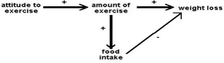
[7][12] [13] [14] Path analysis is a straightforward extension of multiple regressions. Its aim is to provide estimates of the magnitude and significance of hypothesized causal connections between sets of variables. This is best explained by considering a path diagram.

To construct a path diagram we simply write the names of the variables and draw an arrow from each variable to any other variable we believe that it affects. We can distinguish between input and output path diagrams. An input path diagram is one that is drawn beforehand to help plan the analysis and represents the causal connections that are predicted by our hypothesis. An output path diagram

represents the results of a statistical analysis, and shows what was actually found.

So we might have an input path diagram like this:

Figure 1: Idealized input path diagram

And an output path diagram like this:

Figure 2: Idealized output path diagram

It is helpful to draw the arrows so that their widths are proportional to the (hypothetical or actual) size of the path coefficients. Sometimes it is helpful to eliminate negative relationships by reflecting variables - e.g. instead of drawing a negative relationship between age and liberalism drawing a positive relationship between age and conservatism. Sometimes we do not want to specify the causal direction between two variables: in this case we use a double-headed arrow. Sometimes, paths whose coefficients fall below some absolute magnitude or which do not reach some significance level are omitted in the output path diagram.

Some researchers will add an additional arrow pointing in to each node of the path diagram which is being taken as a dependent variable, to signify the unexplained variance - the variation in that variable that is due to factors not included in the analysis.

(3)

correlational data are still correlational. Within a given path diagram, patha analysis can tell us which are the more important (and significant) paths, and this may have implications for the plausibility of pre-specified causal hypotheses. But path analysis cannot tell us which of two distinct path diagrams is to be preferred, nor can it tell us whether the correlation between A and B represents a causal effect of A on B, a causal effect of B on A, mutual dependence on other variables C, D etc, or some mixture of these. No program can take into account variables that are not included in an analysis.

What, then, can a path analysis do? Most obviously, if two or more pre-specified causal hypotheses can be represented within a single input path diagram, the relative sizes of path coefficients in the output path diagram may tell us which of them is better supported by the data.

III. RESULTS

A. brief introduction to SEM with an eating disorder

example:

Now, we present a simple example of SEM.

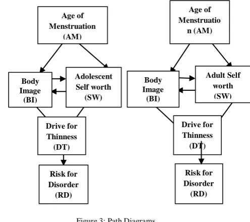
The Hypothesis: We received a hypothesis and data from a psychologist interested in determining what factors in a young woman’s life influence her risk for developing an eating disorder.

“The following path is proposed as a representation of the Relationship and inter-relationships among age of menarche, Press for thinness, body image, and self-concept. Age at onset of menarche will lead to a more negative body image and Self-concept which will lead to an increased press for thinness and an increase in eating disordered symptomatology.”

We can test the validity of her hypothesis using SEM.

a. The Data:

Summary of variables incorporated into the model: a) Age of first menstrual period

b) Body Image score

c) Self Concept score: measured differently for adolescents and for adults, so we have two separate models

d) Drive for thinness

e) Risk for developing an eating disorder

The psychologist evaluated many aspects of each participant’s life and combined the results to create a score for each variable.

B. List wise/Pair wise Deletion:

What do we do when we have missing measurements? There are several ways a researcher can deal with missing data values. Two of them are listed here. In both cases, we assume that any missing data is missing completely at

random. If much data is lost in deletion, imputation should

be considered

List wise: We delete a subject from the study if any of its measurement values are missing.

Pair wise Deletion: We omit those subjects from a particular calculation who do not have the corresponding measurement value. The subjects are present in any calculation for which their value exists.

In our study, we use list wise deletion to delete those subjects

Who do not have the age of first menstrual period

variable? We lose less than 10% of our data in deletion. Creating Two Models: We have two groups of subjects as classified by the grade of the participant. Grade is a variable included in the data but not used in the SEM model, as it was not present in the hypothesis.

If a subject has grade≤ 12, she is an adolescent

If a subject has grade >12, she is an adult.

a. The psychologist in this study first requested two separate models — one for adults and one for adolescents.

For our example Path diagrams are shown as follows.

Figure 3: Path Diagrams

Directional Arrows indicate cause and effect:

Because there are no latent variables, we can write basic regression equations for each variable. Our system is as follows:

The most popular software packages for SEM are: a. LISREL

b. EQS (Peter Bentler) c. AMOS

d. PROC CALIS (and PROC TCALIS) in SAS e. SPSS

(4)

D. ABOUT SAS:

[16]SAS is mainly business analytics software.SAS has delivered proven solutions that drive innovation and improve performance since 1976. SAS has an impact on everyone, every day. From the roads you travel and mortgage loans you purchase, to the brand of cereal you eat and cell phone plan you select, SAS plays a role in your daily life. The SAS language is the general programming language at the heart of SAS software .[17] At many business sites, it has become the predominant programming language for new business applications, largely replacing PL/I, Basic, C, and COBOL. SAS software’s high-level I/O features and its many advanced features for working with data often mean that an application can be developed with a fraction of the coding that a traditional programming language would require. At the same time, SAS’s portability means that SAS programs require surprisingly few changes to move to a different computer or operating system. [18][19]Besides the SAS language itself, SAS software includes routines for doing many of the most common things that people do with data. A SAS program can call on in formats, formats, procs, and other SAS routines to do everything from interpreting data values to applying a statistical test to a set of data.

Developing the same functionality in a standalone programming language such as C would require writing much more code with a much greater potential for error. SAS is computer software for working with data. It has its own programming language, also called SAS, which is the primary way of accessing its features. SAS programs are written not just by professional computer programmers, but also by business analysts, researchers, end users, statisticians, and students. SAS is widely used in big business, financial services, pharmaceutical research, higher education, and government operations. SAS is published by a privately held U.S. company which is also called SAS.[20]SAS has helped organizations across all industries realize the full potential of their greatest asset: data. Simply put, SAS allows you to transform data about customers, performance, financials and more into information and predictive insight that lays the groundwork for solid and coherent decisions. SAS statistical software provides a powerful tool to analyze, manage, view, and even prevent complex data in a variety of formats. SAS Code for our eating disorder is as follows.

Figure: 5 SAS CODE

Here again we use a test and or the confidence intervals to evaluate which paths are significant

(5)

Volume 3, No. 2, March-April 2012

International Journal of Advanced Research in Computer Science

RESEARCH PAPER

Available Online at www.ijarcs.info

ISSN No. 0976-5697

SAS gives us parameter estimates, error estimates and t-values of each path included in the model. We use a t-test to determine which paths are significant. In addition, we can calculate the confidence interval.

If zero is contained in the interval, then the path is not significant.

DT = 0.8285 * BIOSCORE + 0.4255 * AGISelfWorth + 1.0000 * e3

Std Err 0.1430 b5 0.4366 b6

T Value 5.7935 0.9745

EDAC 0.8967 * D7 + 1.0000 e4

Std Err 0.0659 b7

T Value 13.5911

BIQSCORE = -0.239B * AGISelfWorth + - 0.4157 * AgeMenses + 1.0000 e1

Std Err 0.9621 b2 1.2612 b1

T Value -0.3116 -0.3296

AGI Self Worth = 0.1289 * BIOSQUARE + 0.2662 * AgeMenses + 1.0000 e2

Std Err 0.1012 b4 0.3694 b3

T Value -1.2736 0.7206

SAS gives us parameter estimates, error estimates and t-values of each path included in the model. We use a t-test to determine which paths are significant. In addition, we can calculate the confidence interval.

(6)

Figure: 7 Results of SAS Analysis Adolescen#ts

DT = 0.3341 * BIOSCORE + 0.2699 * GISelfWorth + 1.0000 * e3

Std Err 0.1511 b5 0.5396 b6

T Value 2.2112 0.5002

EDAC 0.8292 * DT + 1.0000 e4

Std Err 0.0550 b7

T Value 15.0843

BIQSCORE = -0.0525B * GISelfWorth + - 1.9912 * AgeMenses + 1.0000 e1

Std Err 1.0060 b2 1.0376 b1

T Value -0.0522 -1.9191

AGI Self Worth = 0.1040 * BIOSQUARE + 0.1232 * AgeMenses + 1.0000 e2

Std Err 0.0845 b4 0.3277 b3

T Value -1.2308 0.3758

IV. DISCUSSION

Goodness of Fit

After reporting the parameter estimates, SAS reports many different measures of fit so we can evaluate it in any way we choose. The more measures we use to evaluate our model, the better.

(7)

Fit function 0.2229

Goodness of Fit Index (GFI 0.9257 GFI Adjusted for Degree of Freedom (AGFI) 0.6286 Root Mean Square Residual (RMR) 3.8111 Parsimonious GFI (Mulaik, 1989) 0.2777

Chi-Square 10.0307

Chi-Square DF 3

Pr > Chi-Square 0.0183

Independence Model Chi-Square 107.76 Independence Model Chi-Square DF 10

RMSEA Estimate 0.2282

RMSEA 90% Lower Confidence Limit 0.0827 RMSEA 90% Upper Confidence Limit 0.3913

Adult

Fit function 0.0573

Goodness of Fit Index (GFI) 0.9784 GFI Adjusted for Degree of Freedom (AGFI) 0.8921 Root Mean Square Residual (RMR) 1.6315 Parsimonious GFI (Mulaik, 1989) 0.2935

Chi-Square 1.7177

Chi-Square DF 3

Pr > Chi-Square 0.6330

Independence Model Chi-Square 93.718 Independence Model Chi-Square DF 10

RMSEA Estimate 0.0000

RMSEA 90% Lower Confidence Limit RMSEA 90% Upper Confidence Limit 0.2483

V. CONCLUSION

Our review conﬁrmed that SEM is a highly versatile tool heavily used in the research literature to investigate a variety of problems. Although there are high-quality applications that provide important insights or advances in particular substantive areas,

there are also problematic aspects of this literature. These range from problems of perspective, design, and strategy to mechanical aspects of model speciﬁcation, data analysis, interpretation, and presentation. The problems we have described can have a substantial impact on the quality of information produced in these applications as well as on the validity of interpretations and conclusions.

Paying attention to the concerns raised in this review should enhance the quality of applications of SEM and in turn increase the quality of knowledge gained from its use.

VI. REFERENCES

[1]. G. K. Gupta, “Introduction to Data Mining with Case Studies”, Easter Economy Edition, Prentice Hall of India, 2006 pp. 2-18.

[2]. Jiawei Han and Micheline Kamber, “Data Mining: Concepts and Techniques”, 2nd edition, Morgan Kaufmann Publishers, 2006 pp. 45-70.

[3]. Arun k Pujari ,” Data Mining Techniques” University Press 2009 pp. 62-67.

[4]. Kenneth A. Bollen,”Structural equations with latent Variables”, 1st Edition, Wiley Series in Probability and Mathematical Statistics. New York: John Wiley & Sons, 1989 pp. 306-311.

[5]. Randall Schumacher, Richard G. Lomax, “A Beginner's Guide to Structural Equation Modeling”, 3rd Edition, Psychology Press, 2010 pp. 57-65.

[6]. Pang-Ning Tan, Michael Steinbach, Vipin Kumar, “Introduction to Data Mining”, Addison-Wesley, 2005 pp. 19-36.

[7]. Rex B. Kline, “Principles and Practice of Structural

Equation Modeling”, Guilford Publications, 2004pp. 48-65.

[8]. Geffen, David; Straub, Delmar; and Boudreau, Marie-Claude, "Structural Equation Modeling and Regression Guidelines for Research Practice", 2000, Vol. 4, Issue 7, Communications of the Association for Information Systems, pp. 10-30.

[9]. Barbara M. Byrne, “Structural Equation Modeling With AMOS: Basic Concepts, Applications, and Programming (Multivariate Applications Series)”, 2nd Edition, Mahwah Publishers, New Jersey, 2001 pp. 57-91.

[10]. Anders Skrondal and Sophia Rabe-Hesketh, “Generalized Latent Variable Modeling: Multilevel, Longitudinal, and Structural Equation Models, (Monographs on Statistics and Applied Probability)”, 2nd Edition, 2004 pp. 49-63.

(8)

exponential family”, Issue 4, pp. 515-530.

[12]. I. Garcia Lautre, “A methodology for measuring Latent VariablesBased on multiple factor analysis”, Computational Statistics & Data Analysis, 2004, Volume: 45, Issue: 3, pp. 505-517.

[13].

[14]. John C. Loehlin. Lawrence Erlbaum Associates, “Latent Variable Models: An Introduction to Factor, Path and Structural Equation Analysis”, 4th Edition, Lawrence Erlbaum Associates Publishers, 2004 pp. 8-15.

[15]. Bryman, A. & Cramer, D, “Quantitative data analysis for Social scientists”, 1st Edition, Publisher: Rout ledge; Rev Sub edition. 1994 pp.17.

[16]. Larry Hatcher “A Step-by-Step Approach to Using the SAS System for Factor Analysis and Structural Equation Modeling”, 1st Edition, SAS Publishing, 1994 pp. 57-107,441.

[17]. SAS Institute, “SAS/STAT User’s Guide, Version 6”, 4th Edition, Publisher: SAS Institute, 1990. http://www2.sas.com/proceedings/sugi24/Infovis/p160-24.pdf

[18]. SAS Institute, “SAS Language and Procedures: Usage 2, Version 6”, 1st Edition, SAS Institute Publications, 1990.

[19]. Rebecca J. Elliott “Learning SAS in the Computer Lab”, 2nd Edition, Duxbury Press, 1999 pp. 6-20.