Side Channel Information Set Decoding
using Iterative Chunking
Plaintext Recovery from the “Classic McEliece”
Hardware Reference Implementation
Norman Lahr1, Ruben Niederhagen1, Richard Petri1, and Simona Samardjiska2 1 Fraunhofer SIT, Darmstadt, Germany
[email protected],[email protected],[email protected] 2 Radboud Universiteit, Nijmegen, The Netherlands
Abstract. This paper presents an attack based on side-channel infor-mation and Inforinfor-mation Set Decoding (ISD) on the Niederreiter cryp-tosystem and an evaluation of the practicality of the attack using an elec-tromagnetic side channel. First, we describe a basic plaintext-recovery attack on the decryption algorithm of the Niederreiter cryptosystem. In case the cryptosystem is used as Key-Encapsulation Mechanism (KEM) in a key exchange, the plaintext corresponds to a session key. Our tack is an adaptation of the timing side-channel plaintext-recovery at-tack by Shoufan et al. from 2010 on the McEliece cryptosystem using the non-constant time Patterson’s decoding algorithm to the Niederre-iter cryptosystem using the constant time Berlekamp-Massey decoding algorithm. We then enhance our attack by utilizing an ISD approach to support the basic attack and we introduce iterative column chunking to further significantly reduce the number of required side-channel mea-surements. We theoretically show that our attack improvements have a significant impact on reducing the number of required side-channel measurements. Our practical evaluation of the attack targets the FPGA-implementation of the Niederreiter cryptosystem in the NIST submission “Classic McEliece” with a constant time decoding algorithm and is feasi-ble for all proposed parameters sets of this submission. For example, for the 256bit-security parameter setkem/mceliece6960119we improve the basic attack that requires 5415 measurements to on average of about 560 measurements to mount a successful plaintext recovery attack. Further reductions can be achieved at increasing cost of the ISD computations.
Keywords: ISD · Reaction Attack · SCA · FPGA · PQC · Nieder-reiter · Classic McEliece
1 Introduction
weather forecast [21]. This growing interest in quantum computing has led to a rapid development of quantum computers in the last decade. At the Consumer Electronics Show (CES) in 2019, IBM announced their first commercial quantum computer with 20 qubits [25]. Even larger experimental quantum computers are operating in the labs of Google, IBM, and Microsoft. However, besides the high hopes on a new area of quantum computing, quantum computers pose a severe threat on today’s IT security: A sufficiently large and stable quantum computer can solve the integer factorization and discrete logarithm problems in polyno-mial time using Shor’s quantum-computer algorithm [30, 31], thus completely breaking most of the current asymmetric cryptography like RSA, DSA, and DH as well as ECC schemes like ECDSA, and ECDH.
As an answer to this threat on asymmetric cryptography, the research field of Post-Quantum Cryptography (PQC) has emerged in the last two decades, de-veloping and revisiting alternative cryptographic schemes that are able to with-stand attacks by quantum computers. The most popular approaches are hash-, lattice-, code-, and isogeny-based as well as multivariate cryptography [4, 13]. Hash-based cryptography is used for very reliable signature schemes. Lattice-based cryptography has the reputation of being very efficient. However, code-based cryptography using certain codes is often regarded as already more mature and reliable. Conservative but less efficient examples for code-based cryptogra-phy are the McEliece [24] and the Niederreiter [26] cryptosystems using binary Goppa codes. Multivariate schemes tend to be less popular due to efficiency is-sues. Isogeny-based cryptography is the most juvenile class of PQC and thus not yet fully trusted. In November 2017, the National Institute of Standards and Technology (NIST) started a public process for the standardization of PQC schemes [11]; schemes from all classes mentioned above have been submitted.
An important question in the standardization process besides the definition of secure schemes and the choice of secure parameters is the impact of the imple-mentation of a scheme on its security. A general requirement on the implemen-tation of a scheme is that the runtime of the operations, e.g., key generation, signing, or decryption, does not vary based on secret information like the private key or the plaintext, i.e., that the scheme has a constant-time implementation. (Constant time in regard to public input data like the public key or the cipher-text is not required for this property.) However, there are more side channels besides timing that might enable an attacker to get access to private informa-tion. Other side channels include power consumption and electromagnetic, pho-tonic, and acoustic emission. For many PQC schemes, it is still unknown what side-channel attacks are practically feasible and how to protect against them. A general overview of the state of attacks on the implementation of PQC schemes is presented in [35].
with its name — is using the equivalent approach proposed by Niederreiter as described in Section 2.3.
Our Contributions. We show how to adapt the side-channel attack from Shoufan et al. in [32] for plaintext recovery on the McEliece cryptosystem to a side-channel attack on the Niederreiter cryptosystem. The attack of Shoufan et al. is aiming at a timing side channel due to the non-constant time Patter-son’s decoder, while we perform an EM side-channel attack on the „Classic McEliece” hardware reference implementation [37], which is using a constant time Berlekamp-Massey decoder. If the Niederreiter cryptosystem is used as ba-sis for a KEM in a key exchange, the plaintext constitutes the shared secret that is used to derive a session key. Thus, not just only a single plaintext message can be obtained by the attacker but all following encrypted communication in the session is revealed.
We optimize the number of required side-channel queries using a reaction-based attack combined with a technique that we call iterative chunking. The approach enables us to iteratively increase the number of learned error posi-tions (chunks) in one (cumulative) query. We theoretically estimate the optimal chunk size for an attack based on the system parameters. We further improve our attack by applying known Information Set Decoding (ISD) algorithms and an-alyze the computational cost in relation to the number of required side-channel queries. While using ISD techniques reduces the required number of queries, it comes at a cost of computational power, so the trade-off strongly depends on the computational capabilities of the attacker.
We investigate the hardware implementation by Wang et al. in [37] accom-panying the NIST submission “Classic McEliece” [5] for possible information leakage and we demonstrate the feasibility of our attack exploiting an electro-magnetic field (EM) side channel in that hardware implementation.
Related Work. In [32] a timing attack on the McEliece PKC is presented that recovers the plaintext of a given ciphertext using a decryption oracle. In this attack, a bit-flip error is added to the ciphertext, which results in a shorter timing during decryption, if the flipped bit was set in the original error vector. Fault attacks on the variables used during encryption by McEliece and Niederreiter schemes are examined in [9]. A Differential Power Analysis (DPA) attack is presented in [10] that recovers the secret key of a QC-MDPC McEliece FPGA implementation by measuring the leakage of the carry occuring during the key rotation operation. A similar attack on a software implementation is presented in [13], using the detection of counter overflows. An attack described in [28] uses information gained by DPA about the positions of set bits to recover the secret key in a cryptanalytic attack.
whether these cause decryption failures. Based only on observing whether there was a failure, these attacks can extract the secret key.
Information Set Decoding is a well known decoding technique that is dating back to the work of Prange [27] in the 1960’s. The basic approach has been improved throughout the years by the works of Lee and Brickell [18], Leon [19], Stern [34] (and concurrently Dumer [12]) who first proposed to use collision decoding (actually the term was introduced later [8]). All subsequent improve-ments build on top of Stern’s algorithm by exploring more refined techniques for collision search. The list is extensive and includes: [14, 8, 22, 2, 23].
We are not aware of a previous work that combines information set decoding with side channel analysis and and cumulative reactions.
Structure of this paper. Section 2 provides some background information on in-formation set decoding and on the code-based McEliece and Niederreiter cryp-tosystems and gives a brief introduction to the side-channel attack from Shoufan et al. [32]. Section 3 follows up with a description of our adaption of that at-tack to Niederreiter and our improvements for reducing the number of queries with iterative chunking. Here, we mathematically predict the optimal parame-ter for our chunking strategy, describe an implementation of it using an ideal decryption oracle, and discuss first evaluation results. In Section 4, we provide a leakage analysis of the FPGA implementation from [37] using EM leakage, present a construction of a practical decryption oracle, and evaluate the entire approach practically. Section 5 concludes the paper.
Notation. In the following w(x) denotes the function returning the Hamming weight (HW) of an input vectorx. Capital letters likeH denote matrices. Small
letters denote integer values (e.g.,m,n,k,i,j, andt) or vectors (e.g., plaintextp,
ciphertextc, and error vectore). GF(q)denotes the Galois field of orderq.
2 Background
In this section, we briefly introduce Information Set Decoding, the McEliece cryptosystem and its dual variant the Niederreiter cryptosystem, which will be the object of our attack, as well as the timing attack from Shoufan et al. [32].
2.1 Information Set Decoding
Suppose we are given a parity check matrixH and a syndromes. An ISD
algo-rithm solves the decoding problem:
Find e, w(e) =wsuch that H·e=s. (1)
Basically, the algorithm tries to guess the error vector on k coordinates, and
this set ofkcoordinates theinformation set, since it carries enough information
to recover the entire error vector. The decoding problem gives rise to the system:
H·e=s (2)
with the error coordinatese1, . . . , enas unknowns. Ifkcoordinates are correctly
guessed, the system (2) can be uniquely solved. We check the correctness of the solution by measuring the weight of the error. If the guess was wrong, we guess again.
Information set decoding was proposed by Prange [27]. In this simplest form, we assume an error-free information set. The probability that we guessk
error-free coordinates is n−k w
/ wn. Stern’s variant [34] first introduced collision
de-coding that makes use of the birthday paradox. In essence, we allow some errors in the information set which increases the probability of success. The informa-tion set is split into sets with equal amount of errors p. Then the algorithm
searches for collisions on these two sets, such that the sum of p columns
re-stricted to`coordinates matches the appropriate coordinates of the syndrome.
It is the birthday decoding idea that improves asymptotically with respect to the previous variants. This idea was further generalized in the May-Meurer-Thomae (MMT) [22] and the Becker-Joux-May-Meurer (BJMM) [2] variants that use the more elaborate generalized birthday problem. Here instead of looking for colli-sions between two lists, the collision search is between 4 or 8 lists in multiple layers. May and Ozerov [23] noticed that Stern’s approach can be improved by using more sophisticated algorithms for approximate matching. Their approach is general enough to be applied to other variants such as BJMM.
2.2 McEliece Cryptosystem
In 1978, McEliece proposed a cryptosystem using error correcting codes [24]. The basic idea of this cryptosystem is to use an error correcting code with an efficient error correction algorithm that can correct up tot errors as secret key
and an obfuscated generator matrix of the corresponding code as public key. With code lengthn and code dimensionk, the public key is ak×ngenerator
matrixG. Encryption works by computing a code word for the plaintextpusing
the generator matrix and by adding an errorewith w(e)≤tthat is small enough
so that the error correction algorithm is able to correct the error. The ciphertext
cis therefore computed asc=Gp+e. The receiver simply corrects the error by
applying his secret error correction algorithm and recovers the plaintext from the code word. The security of the system is based on the hardness of decoding a general linear code, a problem known to be NP-hard [3].
2.3 Niederreiter Cryptosystem
In 1986, Niederreiter proposed a dual variant of the McEliece cryptosystem using a (n−k)×n parity-check matrix H instead of a generator matrix as public
syndromec=Heof the error vector is the ciphertext. Here, an efficient syndrome
decoding algorithm is used for decryption. Due to the format requirements on the plaintext of having a certain length and weight, this scheme is usually used as a hybrid scheme with a random error vector that is used with a key derivation function to obtain a symmetric key for the encryption of the actual message.
In general, any error correcting code can be used for the McEliece and Nieder-reiter cryptosystems; however, in order to obtain an efficient and secure system, the code must be efficient to decode with possession of the secret key and hard to decode given only the public key and a ciphertext. McEliece proposed to use binary Goppa codes, which is still considered secure, while Niederreiter origi-nally proposed to use Reed-Solomon codes, which turned out to be insecure [33]. Today, there are many variations of the McEliece and Niederreiter systems us-ing different codes with different properties. However, usus-ing binary Goppa codes (for both McEliece and Niederreiter) is generally the most conservative choice. A drawback of using binary Goppa codes is the large size of the public key of around1 MBfor 256-bit security. In the following, we will focus on the Nieder-reiter cryptosystem with binary Goppa codes with parameters as defined in the NIST submission “Classic McEliece” for Round 1 [5] and Round 2 [6] (see also [7]). We have summarized the notation that we will use in Table 1.
Key generation of the Niederreiter cryptosystem using binary Goppa codes works as follows (following the notation in [36]): Choose a random irreducible polynomialg(x)over GF(2m)of degreetand a list(α
0, α1, . . . αn−1)∈GF(2m)n of distinct elements of GF(2m). From g(x)and (α
0, α1, . . . αn−1), compute the
t×nparity-check matrix H over GF(2m). Transform H into amt×n binary
matrixH0 by replacing each GF(2m)-entry by am-bit column. Finally compute
the systematic form [Imt|K] of H0 and return g(x) and (α0, α1, . . . αn−1) as private key andKas public key. The last step of computing the systematic form
of the binary parity-check matrixH0 compresses the size of the public key from mtnbits tomt(n−mt)bits, because the preceding identity matrixImtdoes not
need to be stored or communicated.
Encryptionworks as follows: The sender constructs thetm×nbinary
parity-check matrix H00 = [Imt|K] by appending K to the identity matrix Imt and
encrypts the error vector e∈GF(2)n (i.e., the plaintext) with w(e) =t to the
syndromes∈GF(2)mt ass=H00e(i.e., the ciphertext).
Decryptionof the syndrome depends on the error-correcting code that is used. Examples are Patterson’s algorithm and the constant-time Berlekamp-Massey (BM) algorithm. Using the BM algorithm as in [7, 37], decryption works as follows: Since the BM algorithm can only correct up tot/2 errors, use the trick attributed to Sendrier in [17] and compute the double-size 2t×n parity-check
matrixH(2)over GF(2m). Then compute the double-size syndromes(2)=H(2)· (s|0) by appending n−mtzeros to the syndrome s. Now, we can use the BM
algorithm to compute the error-locator polynomial σ(x) of s(2). The roots of σ(x)correspond to the error-positions. Therefore, the error-vector bits can be determined by evaluating σ(x) at all points in (α0, α1, . . . αn−1). If σ(αi) =
Symbol Description
m∈N Size of the binary field.
t∈N Correctable errors.
n∈N Code length.
k∈N Code dimension (k=n−mt).
g(x) Goppa polynomial over GF(2m)of degreet.
(α0, α1, . . . αn−1)∈GF(2m)n Support ofndistinct elements of GF(2m). H∈GF(2m)t×n Parity-check matrix.
H0, H00∈GF(2)mt×n Binary parity-check matrix.
H(2)∈GF(2m)2t×n Double-size parity-check matrix. K∈GF(2)mt×(n−mt) Public key.
e∈GF(2)n Error vector (plaintext).
s∈GF(2)mt Syndrome (ciphertext).
s(2)∈GF(2m)2t Double-size syndrome.
σ(x) Error locator polynomial over GF(2m)of degreet.
Table 1.Symbols for Classic McEliece (Niederreiter) [6, 37].
kem/mceliece
-348864 460896 6688128 6960119 8192128
m 12 13 13 13 13
t 64 96 128 119 128
n 3488 4608 6688 6960 8192
k=n−mt 2720 3360 5024 5413 6528
Table 2.Parameter sets of Classic McEliece [6].
A KEM is constructed in “Classic McEliece” from the basic encryption/decryp-tion primitives using a standard transformaencryption/decryp-tion. Table 2 shows the parameters proposed by [6].
2.4 Timing Side-Channel Attack on McEliece
mount the following attack: By iteratively adding an error to each position of the ciphertext and determining via the side channel if in total the number of errors has increased or decreased, the attacker is able to determine the position of all error bits, to correct the errors, and to decode the ciphertext.
Patterson’s algorithm is a popular decoding algorithm for binary Goppa codes. However, the runtime of Patterson’s algorithm depends on the number of errors that have been added to the code word. Shoufan et al. are using these timing variations in Patterson’s algorithm as side-channel information to mount their attack: If an error is added to a previously error-free position, Patterson’s algorithm has a slightly longer runtime; if an error is extinguished by the addi-tional error bit, the runtime of Patterson’s algorithm is slightly shorter. Precisely measuring and categorizing the runtime of Patterson’s algorithm gives the re-quired information to recover the error positions.
3 Reaction-based Side-Channel Analysis
In this section, we describe our reaction-based plaintext-recovery attack on the Niederreiter cryptosystem. We explain how we adapt the timing attack by Shoufan et al. [32] introduced in Section 2.4 on the McEliece cryptosystem to an EM side-channel attack on the Niederreiter cryptosystem in Section 3.1. We describe how to reduce the number of queries required for a side-channel attack when using ISD in Section 3.2 and we improve our basic attack in Section 3.3 using larger chunks in each query. Further, we mathematically predict the op-timal parameter for our query startegy and evaluate its implementation with a simulation using an ideal decryption oracle. Finally, we explain how to combine the ISD techniques with our improved attack in Section 3.4.
3.1 Side-Channel Attack on Niederreiter
Algorithm 1: Iterative Reaction-based SCA input :Classic McEliece parametersn, m, t∈N+,
binary parity-check matrixH00= [Imt|K] := (hi,j)∈GF(2)mt×n, syndromes∈GF(2)mt.
output:Error vectore∈GF(2)n. 1 e←(0, . . . ,0);
2 fori←0ton−1do
3 s0←s⊕H00[i];
4 ifOracle(s0) =truethen e[i]←1;
5 end
6 returne;
query to an oracle is required (line 4 in Algorithm 1) that returns true if the
number is reduced and thus an error position has been found.
This decryption oracle can practically be achieved by having the victim de-crypt the manipulated ciphertext and by measuring the side channel during the decryption. Therefore, when a non-constant time decoding algorithm like Peter-son’s algorithm is used, a timing side-channel attack as in [32] can be mounted on Niederreiter as well.
Attacking constant time implementations. In modern implementations, often a constant time algorithm, typically the Berlekamp-Massey (BM) decoding algo-rithm, is used in order to prevent timing side channels. Thus, in this case another side channel is required to mount the attack. In Section 4, we investigate EM side channels in the reference hardware implementation by Wang et al [37] using the BM algorithm to demonstrate a practical attack. Another side-channel could for example be a response in a communication protocol if adding an error results in a decoding failure and if this failure is reported over the network.
For a side-channel attack based on EM, the attacker needs to be in possession of the device under attack, e.g., a smart card or a security token, that has physical measures protecting secret information such as private and secret keys, but no explicit countermeasures prohibiting the exploitation of the side channel. Furthermore, the attacker needs to be in possession of a ciphertext that she intends to decrypt, e.g., intercepted on a communication channel. Under these requirements, the attacker can perform a series of measurements of EM emissions of the device under attack while decrypting manipulated ciphertexts.
The number of side-channel measurements that is needed for this basic iter-ative attack algorithm is the number of columns n in the parity check matrix,
Algorithm 2: ISD-supported Iterative Reaction-based SCA input :Classic McEliece parametersn, m, t∈N+,
binary parity-check matrixH00= [Imt|K] := (hi,j)∈GF(2)mt×n, syndromes∈GF(2)mt.
output:Error vectore∈GF(2)n. 1 Eb⊂E={1, . . . , n},|Eb|6k;
2 e←(0, . . . ,0);
3 fori∈Ebdo
4 s0←s⊕H00[i];
5 ifOracle(s0) =truethen e[i]←1;
6 end
7 ˜s←s−Hb00·ˆe;
8 ˜e:= (ei)i∈E\
b
E; 9 H˜00:= (hi)i∈E\
b
E; 10 ˆe:= (ei)i∈Eb;
11 ˜e←ISD(n− |Eb|, k− |Eb|, w−w(ˆe),H˜ 00
,˜s);
12 e←Reconstruct(ˆe,˜e);
13 returne;
the attacker to significantly reduce the number of decoding operations that she needs to query from the device under attack.
3.2 Reducing the Number of Queries with Information Set Decoding
The reaction attack described in Algorithm 1 recovers the entire error vector (all error coordinates) using side channel information. Thus, in order to be able to decode, we need to collect at leastn queries from the decryption oracle, which
ranges from3488to8192queries for the NIST parameters of “Classic McEliece” given in Table 2. However, we can reduce the number of queries substantially by focusing on the recovery of an information set of size k < n, instead. Once
an information set is known, we can easily recover the entire error vector using basic linear algebra (see Section 2.1). The information set can be recovered from obtained queries or using some of the ISD algorithms described in Section 2.1. We can also combine the two techniques — first collect a number of queries, use them to reduce the problem to a smaller one, and then solve the smaller problem using an ISD algorithm.
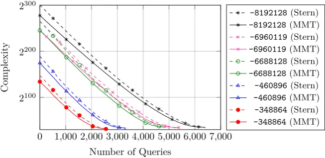
In more detail, let ISD(n, k, w, H, s)be any ISD algorithm, such as Stern’s or Ball Collision decoding, that on input of a parity check matrixH ∈GF(2)(n−k)×n and syndrome s∈GF(2)n−k outputs an error vectore∈GF(2)n — a solution to the decoding problem (1).
0 1,000 2,000 3,000 4,000 5,000 6,000 7,000 2100
2200 2300
Number of Queries
Complexit
y
-8192128(Stern)
-8192128 (MMT)
-6960119(Stern)
-6960119 (MMT)
-6688128(Stern)
-6688128 (MMT)
-460896(Stern)
-460896 (MMT)
-348864(Stern)
-348864 (MMT)
Fig. 1.Time-queries trade-off when using ISD decoding algorithms.
of error indices Eb ⊂ E = {1, . . . , n} We denote the corresponding subvector of e by eˆ= (ei)i∈Eb and its complement by e˜ = (ei)i∈E\Eb. We split similarly
the columns hi = (hj,i)j∈{1,...,mt} of the matrix H00. Let Hb00 = (hi)i∈Eb and
˜
H00 = (hi)i∈E\Eb. With this notation, from the obtained information, we can
transform the decoding problem (1) to: ˜
H00·˜e= ˜s (3)
wheres˜=s−Hb00·ˆe.
So, we have reduced our initial problem to a smaller decoding problem with parametersk0=k− |Eb|,n0 =n− |Eb|,w0=w−w(ˆe). We solve this problem by calling the available ISD algorithm ISD(n0, k0, w0,H˜00,˜s). Note that, if|Eb|=k, we have recovered an information set, and we only need to solve a linear system using Gaussian elimination. Thus, for convention, we assume ISD(n,0, w, H, s) simply performs Gaussian elimination. Algorithm 2 details the whole procedure. The performance of Algorithm 2 depends directly on the size of the setEb, i.e., on the number of queries to the oracle. There is a clear trade-off between the running time and the queries to the oracle, which is depicted in Figure 1. Basically, the attacker is free to choose the number of queries that she performs based on her computational resources.
In our depiction of the trade-off, for simplicity, we used only two ISD algo-rithms — Stern’s and MMT. We did not use the state of the art BJMM variant, because there is no compact representation of the concrete complexity of this algorithm.
(ei, ej) (e0i, e0j)w(e0) Oracle
(0,0) (1,1) w+ 2 false
(0,1) (1,0) w true
(1,0) (0,1) w true
(1,1) (0,0) w−2 true
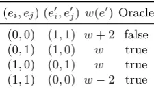
Table 3. All cases of the response of the decryption oracle when querying chunks of size two at once (s0=s⊕hi⊕hj). The first column shows the initial state of the queried chunk, the second column shows the state of the pair after ’flipping’ the values, the third column shows the total number of errors in the new state, and the last column shows the oracle’s answer.
the number of errors has not increased (instead of reduced as in Section 3.1) and false otherwise. Note that the real oracle that we construct in Section 4.2 actually captures both cases.
To get some intuition on how ouriterative chunking works, we first present a simpler variant that already reduces the number of needed queries by more than 35%.
Iterative chunking with β = 2. Suppose that instead of a single error index, we query two error indices (a chunk of sizeβ= 2) at once. We first randomly select the chunk (i, j)of error indices, i, j ∈ {1, . . . , n}, i 6=j. We add both columns hi andhj to the syndromesto obtain the new syndromes0. We give the input
s0 to the decryption oracle. Notice that the decryption oracle will output false
only in the case when the values at corresponding error indices in the error vector were (ei, ej) = (0,0) (a ’low’ chunk). In all the other cases (we refer to
them as ’high’ chunks, to indicate that there is at least one ’1’ in the chunk) the decryption oracle will output true. Indeed, if (ei, ej) = (0,0), after adding the
pair of columns(hi, hj)to the syndrome, we obtain(e0i, e0j) = (1,1), and in total
w+2errors. Hence, the number of errors has increased and the decryption oracle will output false. If (ei, ej) = (0,1) or (ei, ej) = (1,0), we get (e0i, e0j) = (1,0)
and(e0i, e0j) = (0,1)respectively, and in this case the number of errors does not change (it remains w) so the decryption oracle returns true. In the last case,
(ei, ej) = (1,1), after adding the columns we obtain (e0i, e0j) = (0,0). So in this
case, the number of errors reduces to w−2, and the decryption oracle returns true as well. Table 3 summarizes the above.
What we can conclude from the previous is that iffalse is returned, we can be sure that the corresponding error positions in the error vector were(ei, ej) =
(0,0). Since the length of the error vector is much bigger than its Hamming weight, most of the time the randomly chosen chunk will be(ei, ej) = (0,0), and
s s0=s⊕hi
(ei, ej, ek) (e0i, e
0
j, e
0
k) w(e
0
) Oracle w(e0)−1Oracle (0,0,0) (1,1,1) w+ 3 false w+ 2 false (0,0,1) (1,1,0) w+ 1 false w true
(0,1,0) (1,0,1) w+ 1 false w true
(1,0,0) (0,1,1) w+ 1 false w true
(1,1,0) (0,0,1) w−1 true w−2 true
(1,0,1) (0,1,0) w−1 true w−2 true
(0,1,1) (1,0,0) w−1 true w−2 true
(1,1,1) (0,0,0) w−3 true w−4 true
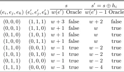
Table 4.Overview of the oracle answers forβ= 3when the number of errors in the
syndrome s are reduced to w(e0)−1 (s0 = s⊕hi) with the knowledge of an error positioniin the original error vectore.
encounterk/2false oracle answers. Note that after a pair has been queried, we need to undo the changes made, i.e., return the pair to its initial state.
Iterative chunking for β >2. This simple strategy for β = 2 is already much better than the naïve approach from the previous paragraph, but we can do much better by extending this idea to chunks (ei1, . . . , eiβ) of size β. We keep the convention of calling the all-zero chunk(0, . . . ,0) ’low’ chunk and all other chunks containing 1s ’high’ chunks. First note that we cannot directly use the same approach for chunks of sizeβ>2. For example forβ= 3we have Table 4 analogous to Table 3.
Table 4 shows (columns 3 and 4) that there is ambiguity in the oracle an-swers, so we can not distinguish whether the chunk was(0,0,0),(0,0,1),(0,1,0) or(1,0,0). However, we can remedy this situation if we reduce the initial num-ber of errors from w to w−1 as columns 5 and 6 from Table 4 show. This requires knowledge about the position of one 1 in the error vector. Adding the corresponding column of the matrixH00to the syndrome reduces the number of errors tow−1. So how can we find the position of one1? Well, this can easily be done by first querying chunks of sizeβ= 2until a ’high’ chunk is found. Query-ing both positions within the ’high’ chunk of size β = 2 reveals the position of one1. The same reasoning extends to any chunk sizeβ: If the number of errors
before we start querying β size chunks isw−(β−2), the oracle answers false only for low chunks, and we can use this information to distinguish low chunks. To summarize, the procedure informally goes as follows: We start with chunk size 2 and continue iteratively. For a chunk size β, we query random chunks
without replacement until the oracle returnstruewhich indicates a ’high’ chunk. Next, we inspect the positions within the ’high’ chunk, and locate the 1s. Now, we can use these1s to increase the size of the chunks that we query: by adding to the syndrome a columnhi of the matrixH00 corresponding to a1at position
iin the error vector we reduce the number of errors by one. This enables us to
only one 1in a ’high’ chunk, so to simplify our analysis we will always increase the size of the queried chunks only by one, although in theory, it is also possible to increase by more than one, precisely by the weight of the ’high’ chunk.
LetE(β)be the expected number of queries on chunks of sizeβuntil we find
a ’high’ chunk (including the query on the ’high’ chunk). Then after this part, we have learnedβ·E(β)error positions — which translates to the same number of new equations for our ISD problem.
Next, we increase the chunk size toβ+ 1, and repeat the same procedure. We could continue increasing the size of the queried chunks until we have learnedk
error positions — enough to recover an information set. However, the increase only makes sense as long as there is a good probability that the queried chunk is ’low’ — in which case one can learnβzeros in the error vector in only one query.
In contrast, if the chunk size is ’high’, since we want to increase the chunk size further, a more expensive inspection with additional queries is required (aroundO(logβ)queries using divide-and-conquer strategy). Thus, if the chunk is ’high’ with big probability, the advantage from the increased chunk size quickly diminishes. Hence, there exists an optimal value for the chunk sizeβ at which
we need to stop increasing. We wil call this threshold value βT. The threshold
βT is an optimization parameter, and we determine its value so that the number
of necessary queries to recover an information set is minimized.
After the threshold is reached, we do not increase the chunk size any more. Now, note the following important observation: Since we do not need to increase the chunk size anymore, it is not essential to find the position of a 1s in the error vector — we only want to find enough ’low’ chunks so that we recover an information set. So in principle, we do not care about ’high’ chunks, unless there are too few chunks remaining — not enough to recover an information set. Therefore, we can safely ignore the ’high’ chunks, but instead of throwing them away, we save them in a bucket of capacity n−k. After the bucket has been
filled, we start inspecting ’high’ chunks as well, because we will not be able to recover an information set otherwise.
The whole procedure ends when we have recoveredkerror positions, i.e. when
we have recovered an information set. The details are given in Algorithm 3. The algorithm for inspecting the ’high’chunks and locating the 1s within the chunk is given in Algorithm 4. It uses a divide and conquer strategy to reduce the number of needed queries.
Find the optimal βT. We next analyze the approach in order to determine the
best threshold value, and estimate the number of queries needed for the attack. First let us make some simple but important observations.
The process of querying chunks of size β can be modeled as a sequence of
Algorithm 3: Iterative Chunking withβ ≥2 input :Classic McEliece parametersn, m, t∈N+,
binary parity-check matrixH00= [Imt|K] := (hi,j)∈GF(2)mt×n, syndromes∈GF(2)mt,
thresholdβT.
output:Partial error vectore0∈GF(2)n,
bucket of chunks containing an error position, list of remaining column indices.
1 e0←[0, . . . ,0]; // initialize with zero vector
2 β←2; // start with chunk size2
3 s0[1]←s;s0[β]←s; // list of syndromess0[i]for each chunk size0< i≤βT 4 indices←[n, . . . ,0]; // column indices in reverse order
5 bucket←[];
6 whileLen(indices)> βdo
7 chunk←Pop(indices, β); // popβ-many indices 8 s00←s0[β] +Sum([H00[i]foriinchunk]) ; // add columns in chunk tos0 9 ifOracle(s00)= truethen // there is an error position 10 ifβ < βT or|bucket|> n−kthen // find errors untilβT is reached 11 eid←FindErrorPositions(chunk, s0, H00); // find errors in chunk
12 foriineiddo
13 e0[i]←1; // updatee0 with found errors 14 ifβ < βT then
15 s0[β+ 1]←s0[β]−H00[i]; // remove found errors froms0 16 β←β+ 1; // increase chunk size, up toβT
17 end
18 else
19 bucket←bucket+chunk; // collect chunks with remaining errors 20 end
21 returne0,bucket,indices;
Based on these observations, we have the following results. The proofs are given in Appendix A.
Proposition 1. Suppose we query chunks of size β without replacement, until
we find a ’high’ chunk.
a. Letpβ denote the probability that the queried chunk is high.
pβ= 1− n−w
β
n β
b. The expected number of queries until we find a ’high’ chunk of sizeβ is:
E(β) = 1
pβ
Algorithm 4: FindErrorPositions input :chunk∈Ni,
list of temporary syndromess0withs[i]∈GF(2)mt,
binary parity-check matrixH00= [Imt|K] := (hi,j)∈GF(2)mt×n. output:List with error indices.
1 stack←[Left(chunk),Right(chunk)];
2 eid←[];
3 whilestacknot empty do 4 chunk←Pop(stack);
5 s00←s0[Len(chunk)] +Sum([H00[i]foriinchunk]);
6 ifOracle(s00)= truethen next←chunk ; // there is an error position 7 else next←Pop(stack) ; // continue search in the stack head
8 ifLen(next)= 1 then // found an error position
9 Push(eid, next[0]);
10 stack←[Flatten(stack)]; // inspect entire stack
11 else // split the next chunk directly
12 Push(stack,Left(next)); 13 Push(stack,Right(next)); 14 end
15 returneid;
c. Let Pr(w(β) =j|High) denote the probability that the weight of the chunk isj under the condition that it is a ’high’ chunk. Then,
Pr(w(β) =j|High) =
w j
n−w β−j
n β
− n−βw. (5)
d. The expected weight of the ’high’ chunk of sizeβ is
E(w(β)) = w
n−1
β−1
n β
− n−βw. (6)
Proposition 1 estimates the number of needed queries to find a ’high’ chunk of size β as well as the expected weight of the found chunk. We should also
estimate the number of queries to inspect a ’high’ chunk, i.e. to determine all error positions within the ’high’ chunk. Various strategies can be applied for this task, which mainly depend on the expected weight of a ’high’ chunk. The simplest one is to just query all positions, which requiresβqueries, but this would
this smaller chunk. The details are given in Algorithm 4. Proposition 2 estimates the number of queries needed to inspect a ’high’ chunk using this algorithm. The proof is given in Appendix A.
Proposition 2. Suppose we inspect a ’high’ chunk of sizeβ. Then, the expected
number of queries to learn all positions within ’high’ chunk of size β using
Algorithm 4 is bounded from above by:
EHigh(β)6 β
X
j=1 (
w j
n−w β−j
n β
− n−βw)·(j−
j β +
j−1 X
i=0
log2(β−i)). (7)
Using Propositions 1 and 2 we can now estimate the number of queries re-quired in Algorithm 3.
Recall that Algorithm 3 first queries chunks of size2, . . . , βT by iteratively
increasing the chunk size right after a ’high’ chunk has been found. As introduced earlier, letE(β)denote the expected number of queries needed to find a ’high’ chunk of sizeβ. Then, the number of error positions that we learn at this step
isβE(β). Repeating the same for chunk sizes2,3. . . , βT−1, we learn a total of
I1(βT) = βT−1
X
i=2
i·E(i) (8)
error positions.
When we reach the threshold valueβT we change the strategy, and continue
to query only chunks of sizeβT. Since we do not need to increase the chunk size,
we do not inspect ’high’ chunks, but save them in a bucket of capacity n−k.
Once the bucket is full we start also inspecting the ’high’ chunks, since otherwise we will not be able to recover an information set (that is of sizek). Suppose we
queryN1·E(βT)chunks while the bucket is sill not full andN2·E(βT)chunks
after the bucket is full, for some unknownN1, N2. The number of learned error positions is
I2(βT) =N1·βT ·(E(βT)−1) +N2·βT·E(βT) (9)
The algorithm stops when k error positions have been learned, i.e. when the
condition
I1(βT) +I2(βT)>k (10)
is satisfied. Since the bucket has capacityn−kwe also have the condition
N1·βT 6n−k (11)
Since the algorithm proceeds until the information set is found or the bucket is full, from equations (10) and (11) we findN1and N2as:
N1=min{
n−k βT
, k−I1(βT) βT ·(E(βT)−1)
} (12)
N2=
I2(βT)−N1·βT ·(E(βT)−1)
βT ·E(βT)
Now it is easy to calculate the number of queries for a given thresholdβT.
Where
Q1(βT) = βT−1
X
i=2
(E(i) +EHigh(i)) (14)
Q2(βT) =N1·E(βT) +N2·(E(βT) +EHigh(βT)) (15)
are the required queries that correspond toI1(βT)and I2(βT) respectively, the
total number of queries is
Q(βT) =Q1(βT) +Q2(βT) (16)
The optimalβT is then the one that minimizes the number of queriesQ(βT).
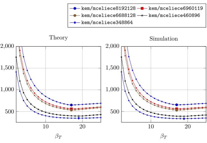
Evaluation. The results of the mathematical prediction and a simulation are depicted in Figure 2. We computed the expected number of queries for βT ∈
{2, . . . ,25}for the parameter setskem/mceliece348864,kem/mceliece460896,
kem/mceliece6688128, kem/mceliece6960119, and kem/mceliece8192128 of “Classic McEliece” (see Table 2). In addition, we implemented the described iterative chunking strategy using Python and SageMath. We ran this imple-mentation as a simualtion with a ideal oracle which always returns the correct response. The simulation was applied to ten different key pairs using ten differ-ent plain-/ciphertext pairs for each key pair (100in total) per parameter set and
βT value. We generated the key pairs as well as the plain- and ciphertext pairs
using the SageMath scripts that are enclosed with the publicly available FPGA implementation of the Niederreiter cryptosystem from Wang et al.
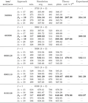
The optimal threshold values for the parameter sets together with the number of needed queries are given in Table 5. The results of the simulation and the later experiments in Section 4.3 show that the estimate matches very well. The number of traces are decreased to approximately12.3%forkem/mceliece348864 down to10%forkem/mceliece8192128compared to the ISD-supported iterative approach in Algorithm 2. As predicted, the number of traces depends on the choice of the chunk size thresholdβT. A smaller chunk size causes more queries.
If the chunk size is too large, the bucket gets filled up with not inspected, as ’high’ responded queries. Thus, additional traces have to be acquired to collect enough columns to apply a plain ISD. We could also spend more computing power to apply Stern or MMT as mentioned above to lower the number of traces further. For the parameter set kem/mceliece460896, in the simulation βT = 18
turned out to be slightly more efficient than the expectedβT = 19. However, we
believe that this is only because the number of queries forβT = 18andβT = 19
in the theoretical prediction are very close to each other.
10 20 500
1,000 1,500 2,000
βT
Theory
10 20
500 1,000 1,500 2,000
βT
Simulation
kem/mceliece8192128 kem/mceliece6960119
kem/mceliece6688128 kem/mceliece460896
kem/mceliece348864
Fig. 2.The expected number of queries needed for threshold values from 2 to 25 both for the theoretical prediction and averaged simulations. The minima are marked.
set from queries, we can stop early, when we have learned only δ < k error
coordinates. Assume at this point we haven0 columns remaining, the weight of
the error vector on these coordinates is w0 and we need to recoverk0 =k−δ
more elements from the information set.
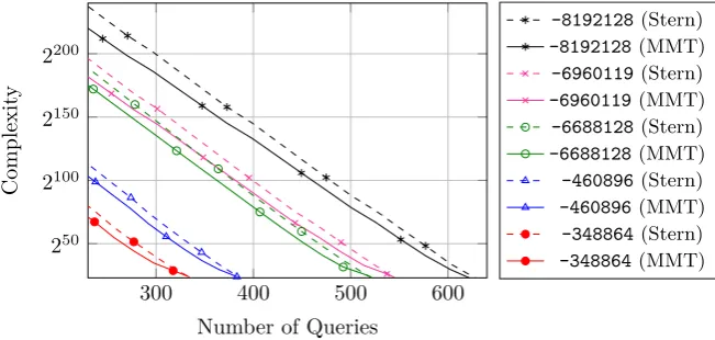
Then we are left with the decoding problem with parameters(n0, k0, w0)which we can solve using any ISD algorithm. Of course this comes with a price since ISD algorithms are exponential in time. Finding the right trade-off depends on the computational power (CPU hours) the attacker has at hand. Figure 3 gives the trade-off when using Stern’s or MMT algorithm. A comparison to plain ISD can also be found in Table 5.
4 Attack Evaluation
300 400 500 600 250
2100
2150 2200
Number of Queries
Complexit
y
-8192128(Stern)
-8192128 (MMT)
-6960119(Stern)
-6960119 (MMT)
-6688128(Stern)
-6688128 (MMT)
-460896(Stern)
-460896 (MMT)
-348864(Stern)
-348864 (MMT)
Fig. 3.Time-queries trade-off when using ISD decoding algorithms.
4.1 Leakage Analysis
To construct a decryption oracle for our attack approach we investigated the implementation by Wang et al. from [37] in detail to find a proper point of interest at which we can find significant leakage. The selected implementation uses the constant-time BM algorithm for the error correction. The BM algorithm returns an error-locator polynomial which has roots at the points that correspond to an error position. Thus, if there aret0 ≤t errors,t0 input points to the error-locator polynomial evaluate to zero. If the number of errors is larger than t, a
random polynomial is returned by the BM algorithm, which most likely has a very small number of roots. Thus, in order to distinguish whether the number of errors has increased or decreased, we need to distinguish cases where the reconstructed error vector has a low HW (for cases with an increased error number where error correction failed) and where it has a high HW (for cases with a decreased error number where error correction succeeded).
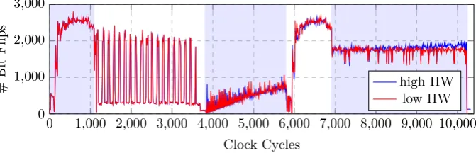
The FPGA implementation of the decryption module in [37] consists of five major steps: First, an additive Fast Fourier Transformation (FFT) evaluates the secret Goppa polynomial. Then the double syndrome is computed. Afterwards the BM algorithm is performed and another additive FFT is applied to evaluate the error-locator polynomial. In the final step, the error vector is constructed.
0 1,000 2,000 3,000 4,000 5,000 6,000 7,000 8,000 9,000 10,000 0
1,000 2,000 3,000
Clock Cycles
#
Bit
Filps
high HW low HW
Fig. 4.Simulated power consumption based on a Hamming-distance model for success-ful decoding (high HW in the resulting error vector) and unsuccesssuccess-ful decoding (low HW) using a small parameter set withm= 12,t= 66, andn= 3307. The different
parts of the algorithm can clearly be seen (marked with alternating blue background color). In the first block, an additive FFT is performed for evaluating the secret Goppa polynomial. In the second block, the double syndrome is computed. In the third block, BM is performed. In the fourth block, another additive FFT is performed in order to evaluate the error-locator polynomial. Finally, the error vector is constructed. A clear difference in the simulation is visible in the last step for the low and high HW results.
at which side-channel information is leaked is at the last round of the second additive FFT operation which evaluates the error-locator polynomial from the BM decoder. The result of this evaluation equals to zero if there is a root and results in other values if not. Thus, it is distinguishable in general. However, because the implementation of the additive FFT utilizes several multiplicator instances in parallel, the logical noise added to the exploitable leakage is quite high.
The second point is at the last step, the error vector construction. Here, the graph of the high HW error vector (blue) increases during the construction in contrast to the low HW error vector (red) such that there is a growing distance between them. The reason for the increasing number of bit flips at this stage is that the result of the error vector construction is shifted into a large flip-flop shift-register step by step. To lower the effort compared to the analysis of the second FFT we exploit the significant leakage of the iterative reconstruction at the end of the decryption process. Therewith, the side-channel information enables the construction of a decryption oracle.
4.2 Building an Oracle in Practice
We decided to use the electromagnetic radiation (EMR) leakage emanated by the FPGA during the decryption and developed a Differential Electromagnetic Analysis (DEMA). Power leakage could be exploited in the same way.
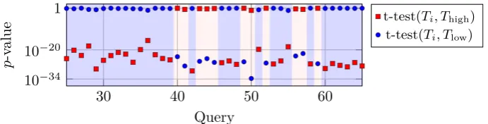
30 40 50 60 10−34
10−20
1
Query
p
-v
alue
t-test(Ti, Thigh) t-test(Ti, Tlow)
Fig. 5.Examplep-values of the t-tests of consecutive oracle queries. For each query a traceTi is compared to a known faulty (Tlow) and a known decodable trace (Thigh). If a trace is similar to the faulty trace (i.e. due to a higherp-value), a decoding failure is detected (light blue background). In the opposite case (light red background) the syndrome could be decoded.
range against two known reference traces. The reference traces stem from de-ciphering the original syndrome for which we know that it is decodable, and from a faulty syndrome that includes more than t errors so that it cannot be
decoded. This has the disadvantage that it adds an overhead of two traces to the total number of required traces. Alternatively, we could statistically deter-mine a threshold to compare it to the result of a t-test with just one of the reference traces, which would save one trace. However, we decided to spend one additional trace and avoid the statistical computation. The faulty syndrome is constructed by adding five columns randomly chosen from the public key ma-trix H00. The probability that this results in syndrome with more errors than can be corrected is high; nevertheless, we use a t-test comparison to the trace of the original syndrome to ensure this requirement. Algorithm 5 details the preparation procedure. Now, we take the difference of the p-values of the t-tests comparing a traceTi against the original syndrome traceThigh and against the
faulty syndrome traceTlow:
p∆=t-test(Ti, Thigh)−t-test(Ti, Tlow) (17)
Thus, if the difference of the p-valuesp∆ is positive the acquired trace is similar
to the original syndrome trace and interpreted as decodable. Otherwise, if p∆
becomes negative it is interpreted as not decodable. Figure 5 gives an example section of p-values of consecutive oracle queries. The response when used as
decryption oracle therefore is:
response= (
true(decodable), ifp∆>0
f alse(not decodable), otherwise (18)
Algorithm 5: GetReferences
input :Classic McEliece parametersn, m, t∈N+,
binary parity-check matrixH00= [Imt|K] := (hi,j)∈GF(2)mt×n, syndromes∈GF(2)mt.
output:Reference tracesThigh0 , T
0
low. 1 Decrypt(s) Thigh, Clkhigh;
2 Thigh0 ←Compress(Thigh, Clkhigh); 3 s∗←s;
4 repeat
5 fori←0to5do
6 i∈R{
0. . . n};
7 s∗←s∗⊕H[i];
8 end
9 Decrypt(s∗) Tlow, Clklow; 10 Tlow0 ←Compress(Tlow, Clklow); 11 untilt-test(Thigh0 , T
0
low)≈0; 12 returnThigh0 , T
0
low;
Algorithm 6: DEMA-based Oracle
input :Manipulated syndromes0∈GF(2)mt, reference tracesThigh0 , T
0
low. output:Oracle response.
1 Decrypt(s0) Tj, Clkj; 2 Tj0←Compress(Tj, Clkj); 3 p∆←t-test(Tj0, T
0
high)−t-test(T
0
j, T
0
low); 4 return
(
true ifp∆>0
f alse otherwise;
as described in [20]. We reduce the raw signal to the maximum peak-to-peak difference of the amplitudes of the EM signal in each first clock half-wave and take it as the new value for the entire clock cycle. We just need to know the set clock frequency of24 MHzto identify the clock cycle ranges in the raw signal.
Optimization. The quality metric of the side channel oracle is the difference of the p-valuesp∆. The greater the absolute value is the better is the differentiability of
the ”low” and the ”high” case. The more errors are removed from the syndrome during the iterative chunking process the less ’1’s are in the resulting error vector and its weight decreases. Since we are using the Hamming weight of the error-vector construction as the exploitable leakage, |p∆| decreases during the
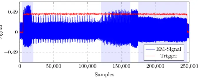
0 50,000 100,000 150,000 200,000 250,000 −0.49
0 0.49
Samples
Signal
EM-Signal Trigger
Fig. 6.Example EM trace of the decryption process on a SAKURA-X (Xilinx Kintex-7, XC7K160T). The five steps (additive FFT, double syndrome computation, Berlekamp-Massey, additive FFT, error vector construction) are highlighted with alternating blue background color as in Figure 4.
4.3 Practical Evaluation
To evaluate the attack in practice, we ported the FPGA design of [37] to a Xilinx Kintex-7 (XC7K160T) on a SAKURA-X3 board running at 24 MHz clock
fre-quency. We added a UART communication interface, a control unit that handles the storage of the secret key parts(g(x),(α0, α1, . . . αn−1)), and a trigger signal to one of the output ports that indicates the start and the end of a decryption operation. We acquired the EMR profiles and the trigger signal using a Pico-Scope 5244D MSO oscilloscope at 500 MSamples/sand a near-field probe from Langer (RF-U 5-2). We added a 10 MHzhigh-pass filter to remove noise in the lower frequency range and used a customized Python script for an automatic acquisition and analysis process. The ISD-support was implemented using the GF(2) arithmetic of SageMath4.
We analyzed the design of the Niederreiter decryption for all parameter sets proposed for “Classic McEliece” in the second round of the NIST PQC com-petition (see Table 2). Figure 6 shows an example trace of a decryption run. Corresponding to the simulated trace in Figure 4, the five individual parts of the decryption process are identifiable.
We evaluated the ISD-supported iterative approach (Section 3.2) and the chunk-based approach (Section 3.3) using the oracle described in Algorithm 6 for all parameter sets. We are using plain ISD (Prange) as ISD algorithm, replacing the “guessing” with queries to our oracle, effectively implementing the ISD as Gaussian elimination on n−k columns that are collected in the bucket. If an
attacker is able to invest some computing power, he is able to reduce the number of traces even further, trading in a higher complexity of the ISD.
We are using the same implementation of the iterative chunking as the sim-ulation described in Section 3.3 — however, we substituted the perfect oracle with the real side-channel oracle described in Algorithm 6. We examined the same data sets as used for the simulation, i.e., ten different key pairs using ten different plain-/ciphertext pairs for each key pair (100 in total) per parameter set. To demonstrate the feasibility of the side-channel-based oracle, we ran the practical evaluation of the plaintext recovery attack for the optimal chunk size threshold (βT) that was determined from the simulation (see Table 5).
For each “Classic McEliece” parameter set of the second round of the NIST competition, we were able to recover the entire plaintexts with our iterative chunking approach. Since the responses of the side channel oracle and the ideal oracle in the simulation are equal, we get the same average number of traces for the same value ofβT in the simulation as well as the experiments.
5 Conclusion
In this paper we presented a side-channel information-based plaintext recov-ery attack against the Niederreiter cryptosystem and specifically the “Clas-sic McEliece” NIST submission. We introduced a novel reaction attack using an iterative chunking strategy and basic Information Set Decoding which en-ables the comulative recovery of error vector values within a single decryp-tion oracle request. This approach decreases the required oracle requests to approximately 12.3% for kem/mceliece348864 (335 traces) down to 10% for kem/mceliece8192128(654 traces) compared to the simple ISD-supported iter-ative approach which requiresk+ 2requests.
We mathematically predict the optimal value for the parameter βT which
is used in the iterative chunking. We implemented the chunking strategy and exhaustively simulate the approach for multiple values using an ideal decryption oracle. The simulated results meet the predicted values very well. Addition-ally, we successfully demonstrated the feasibility of the attack for all proposed parameter sets of the second round using EM side-channel leakage from the ref-erence FPGA implementation of the “Classic McEliece” submission which uses a Berlekamp-Massey decoder.
kem/ Approach Simulation Theory Experiment
mceliece- min. avg. max. plain cost≈240
348864
β= 1 – 2722 (k+ 2) –
βT= 17 281 335.89 483 346.17 — —
βT= 18 275 334.51 481 345.16 — —
βT=19 273 334.16 481 345.06 287.26 334.16
βT= 20 279 337.36 494 345.74 — —
βT= 21 282 337.92 482 347.09 — —
460896
β= 1 – 3362 (k+ 2) –
βT= 16 353 397.01 523 404.41 — —
βT= 17 343 391.72 513 400.00 — —
βT=18 337 389.33 514 396.95 — 389.33
βT=19 333 390.33 515 395.06 337.66 —
βT= 20 329 392.14 517 396.62 — —
βT= 21 326 399.59 532 403.45 — —
6688128
β= 1 – 5026 (k+ 2) –
βT= 15 505 553.56 608 556.73 — —
βT= 16 480 540.10 598 544.22 — —
βT=17 468 532.11 595 534.14 470.91 532.11
βT= 18 456 534.30 604 535.31 — —
βT= 19 448 540.46 617 543.39 — —
6960119
β= 1 – 5415 (k+ 2) –
βT= 15 529 584.15 708 585.21 — —
βT= 16 518 569.93 692 571.24 — —
βT=17 505 561.29 680 559.87 493.90 561.29
βT= 18 508 562.15 679 561.61 — —
βT= 19 499 567.68 685 567.58 — —
8192128
β= 1 – 6530 (k+ 2) –
βT= 15 618 679.41 788 676.59 — —
βT= 16 596 661.87 771 658.28 — —
βT=17 587 653.97 760 648.66 576.96 653.97
βT= 18 571 654.86 760 652.85 — —
βT= 19 586 658.33 778 657.53 — —
Table 5.Statistical data for the required number of queries for a successful recovery of an entire error vector. The data for the simulation and the experiments was gathered from the same sets of ten different key pairs and ten different plain-/ciphertexts per key pair (100in total) for each parameter set. We also give the theoretical prediction
and the number of required queries for applying ISD at a cost of around240operations.
For comparison, we also give the number of traces when no chunking is used, i.e.,β= 1
A Appendix
A.1 Proof of Proposition 1
a. Since the probability of hitting a low chunk is Pr(Low) = ( n−w
β )
(n β)
, we obtain
pβ= 1− n−w
β
n β
.
b. LetPr(w(β) =j|High)denote the probability that the weight of the chunk isj under the condition that it is a high chunk. Then,
Pr(w(β) =j|High) = Pr(w(β) =j)
pβ
.
SincePr(w(β) =j) =( w j)(
n−w β−j) (n
β)
we obtainPr(w(β) =j|High) =
w j
n−w β−j
n β
− n−w β
.
c. Since the querying of chunks of sizeβ follows the geometric distribution, we
immediately obtain the claim. d. From a. we can directly calculate
E(w(β)) =
β
X
j=1
j·Pr(w(β) =j|High) = n 1
β
− n−βw
β X j=1 j· w j
n−w
β−j
=
= n 1
β
− n−βw
β
X
j=1
w·
w−1
j−1
n−w
β−j
= n w
β
− n−βw n−1
β−1
.
A.2 Proof of Proposition 2
To estimateEHigh(β), we will first write it as
EHigh(β) = β
X
j=1
Pr(w(β) =j|High)·EHigh(β|w(β) =j),
where EHigh(β|w(β) = j) denotes the expected number of queries to learn all
positions within a high chunk of sizeβ under the condition that there are exactly j 1s in the chunk.
We consider first EHigh(β|w(β) = 1). Note that we need log2β queries to locate the 1, and on average 1−1/β additional queries for the remaining
un-queried positions. Here=−1/β comes from the case where the 1 is on the last
ForEHigh(β|w(β) = 2)we have:
EHigh(β|w(β) = 2)
= 1β 2
X
16i,j6β
j6=β
(log2β+ log2(β−i) + 2) + 1β 2
X
16i,j6β
j=β
(log2β+ log2(β−i) + 1)
= 1β 2
X
16i,j6β
(log2β+ log2(β−i)) + 2−
β−1 1
β
2
6 1β
2
X
16i,j6β
(log2β+ log2(β−1)) + 2− 2
β = log2β+ log2(β−1) + 2−
2
β
where the second sum in the first row comes from the fact that if the second 1 is on the last position, we need one less query. We boundEHigh(β|w(β) = 2)from
above, instead of calculating it exactly, in order to simplify the expression and the analysis. It is a rather tight bound, which can be confirmed by the simulation and experiments we have performed (see Table 5).
Using induction it is easy to show that
EHigh(β|w(β) =j) = j−1 X
i=0
log2(β−i) +j− j β
Finally,Pr(w(β) =j|High) can be easily calculated from Proposition 1, which gives the final expression.
Acknowledgements
This work has been supported by the European Commission through the ERC Starting Grant 805031 (EPOQUE). Furthermore, this research work has been funded by the German Federal Ministry of Education and Research and the Hes-sen State Ministry for Higher Education, Research and the Arts within their joint support of the National Research Center for Applied Cybersecurity ATHENE.
References
[1] N. Aragon and P. Gaborit. “A key recovery attack against LRPC using de-cryption failures”. In:International Workshop on Coding and Cryptography – WCC 2019. 2019.
[2] A. Becker, A. Joux, A. May, and A. Meurer. “Decoding Random Binary Linear Codes in 2n/20: How 1 + 1 = 0 Improves Information Set Decoding”. In:Advances in Cryptology – EUROCRYPT 2012. Ed. by D. Pointcheval and T. Johansson. Vol. 7237. LNCS. Springer, 2012, pp. 520–536.
[4] D. J. Bernstein, J. Buchmann, and E. Dahmen, eds.Post-Quantum Cryp-tography. Springer, 2009.isbn: 978-3-540-88702-7.
[5] D. J. Bernstein, T. Chou, T. Lange, I. von Maurich, R. Misoczki, R. Nieder-hagen, E. Persichetti, C. Peters, P. Schwabe, N. Sendrier, J. Szefer, and W. Wang.Classic McEliece: conservative code-based cryptography — Round 1. https://classic.mceliece.org/nist/mceliece-20171129.pdf. Nov. 2017.
[6] D. J. Bernstein, T. Chou, T. Lange, I. von Maurich, R. Misoczki, R. Nieder-hagen, E. Persichetti, C. Peters, P. Schwabe, N. Sendrier, J. Szefer, and W. Wang.Classic McEliece: conservative code-based cryptography — Round 2. https://classic.mceliece.org/nist/mceliece-20190331.pdf. Mar. 2019.
[7] D. J. Bernstein, T. Chou, and P. Schwabe. “McBits: fast constant-time code-based cryptography”. In:Cryptographic Hardware and Embedded Sys-tem – CHES 2013. Ed. by G. Bertoni and J.-S. Coron. Vol. 8086. LNCS. Springer, 2013, pp. 250–272.
[8] D. J. Bernstein, T. Lange, and C. Peters. “Smaller Decoding Exponents: Ball-Collision Decoding”. In: Advances in Cryptology – CRYPTO 2011. Ed. by P. Rogaway. Vol. 6841. LNCS. Springer, 2011, pp. 743–760. [9] P.-L. Cayrel and P. Dusart. “McEliece/Niederreiter PKC: Sensitivity to
Fault Injection”. In: 5th International Conference on Future Information Technology. IEEE, 2010, pp. 1–6.
[10] C. Chen, T. Eisenbarth, I. von Maurich, and R. Steinwandt. “Horizontal and Vertical Side Channel Analysis of a McEliece Cryptosystem”. In:IEEE Trans. Inform. Forensics Security 11.6 (2016), pp. 1093–1105.
[11] L. Chen, D. Moody, and Y.-K. Liu. Post-Quantum Cryptography. NIST, https://csrc.nist.gov/Projects/post-quantum-cryptography. [12] I. I. Dumer. “Two Decoding Algorithms for Linear Codes”. In: Probl.
Peredachi Inf.25 (1 1989), pp. 24–32.
[13] L. D. Feo, D. Jao, and J. Plût. “Towards quantum-resistant cryptosystems from supersingular elliptic curve isogenies”. In:J. Mathematical Cryptology 8.3 (2014), pp. 209–247.
[14] M. Finiasz and N. Sendrier. “Security Bounds for the Design of Code-Based Cryptosystems”. In: Advances in Cryptology – ASIACRYPT 2009. Ed. by M. Matsui. Vol. 5912. LNCS. Springer, 2009, pp. 88–105.
[15] Q. Guo, T. Johansson, and P. Stankovski. “A Key Recovery Attack on MDPC with CCA Security Using Decoding Errors”. In:Advances in Cryp-tology – ASIACRYPT 2016. Ed. by J. H. Cheon and T. Takagi. Vol. 10031. LNCS. Springer, 2016, pp. 789–815.
[17] S. Heyse and T. Güneysu. “Code-based cryptography on reconfigurable hardware: tweaking Niederreiter encryption for performance”. In: JCEN 3.1 (2013), pp. 29–43.
[18] P. J. Lee and E. F. Brickell. “An Observation on the Security of McEliece’s Public-Key Cryptosystem”. In: Advances in Cryptology - EUROCRYPT 1988. Ed. by C. G. Günther. Vol. 330. LNCS. Springer, 1988, pp. 275–280. [19] J. S. Leon. “A probabilistic algorithm for computing minimum weights of large error-correcting codes”. In:IEEE Trans. Information Theory34.5 (1988), pp. 1354–1359.
[20] S. Mangard, E. Oswald, and T. Popp.Power Analysis Attacks: Revealing the Secrets of Smart Cards (Advances in Information Security). Springer, 2007.isbn: 978-0-387-30857-9.
[21] B. Marr.6 Practical Examples Of How Quantum Computing Will Change Our World. Forbes, https://www.forbes.com/sites/bernardmarr/ 2017/07/10/6-practical-examples-of-how-quantum-computing-will-change-our-world/. 2017.
[22] A. May, A. Meurer, and E. Thomae. “Decoding Random Linear Codes in ˜
O(20.054n)”. In:Advances in Cryptology – ASIACRYPT 2011. Ed. by D. H. Lee and X. Wang. Vol. 7073. LNCS. Springer, 2011, pp. 107–124.
[23] A. May and I. Ozerov. “On Computing Nearest Neighbors with Applica-tions to Decoding of Binary Linear Codes”. In: Advances in Cryptology – EUROCRYPT 2015. Ed. by E. Oswald and M. Fischlin. Vol. 9056. LNCS. Springer, 2015, pp. 203–228.
[24] R. J. McEliece. “A Public-Key Cryptosystem Based On Algebraic Coding Theory”. In:DSN Progress Report 42–44 (1978), pp. 114–116.
[25] C. Nay. IBM Unveils World’s First Integrated Quantum Computing Sys-tem for Commercial Use. IBM News Roomm https://newsroom.ibm. com/2019-01-08-IBM-Unveils-Worlds-First-Integrated-Quantum-Computing-System-for-Commercial-Use. 2019.
[26] H. Niederreiter. “Knapsack-type cryptosystems and algebraic coding the-ory”. In: Probl. Control Inform.15 (1986), pp. 19–34.
[27] E. Prange. “The use of information sets in decoding cyclic codes”. In:IRE Trans. Information Theory 8.5 (1962), pp. 5–9.
[28] M. Rossi, M. Hamburg, M. Hutter, and M. E. Marson. “A Side-Channel Assisted Cryptanalytic Attack Against QcBits”. In: Cryptographic Hard-ware and Embedded Systems – CHES 2017. Ed. by W. Fischer and N. Homma. Vol. 10529. LNCS. Springer, 2017, pp. 3–23.
[29] S. Samardjiska, P. Santini, E. Persichetti, and G. Banegas. “A Reaction Attack Against Cryptosystems Based on LRPC Codes”. In: Progress in Cryptology – LATINCRYPT 2019. Ed. by P. Schwabe and N. Thériault. Vol. 11774. LNCS. Springer, 2019, pp. 197–216.
[31] P. W. Shor. “Polynomial-time algorithms for prime factorization and dis-crete logarithms on a quantum computer”. In: SIAM review 41.2 (1999), pp. 303–332.
[32] A. Shoufan, F. Strenzke, H. G. Molter, and M. Stöttinger. “A Timing Attack against Patterson Algorithm in the McEliece PKC”. In: Informa-tion, Security and Cryptology – ICISC 2009. Ed. by D. Lee and S. Hong. Vol. 5984. LNCS. Springer, 2010, pp. 161–175.
[33] V. M. Sidelnikov and S. O. Shestakov. “On insecurity of cryptosystems based on generalized Reed-Solomon codes”. In: Discrete Math. Appl. 2.4 (1992), pp. 439–444.
[34] J. Stern. “A method for finding codewords of small weight”. In: Coding Theory and Applications. Ed. by G. Cohen and J. Wolfmann. Vol. 388. LNCS. Springer, 1989, pp. 106–113.
[35] M. Taha and T. Eisenbarth. Implementation Attacks on Post-Quantum Cryptographic Schemes. Cryptology ePrint Archive, Report 2015/1083. [36] W. Wang, J. Szefer, and R. Niederhagen. “FPGA-based Key Generator
for the Niederreiter Cryptosystem Using Binary Goppa Codes”. In: Crypto-graphic Hardware and Embedded Systems – CHES 2017. Ed. by W. Fischer and N. Homma. Vol. 10529. LNCS. Springer, 2017, pp. 253–274.
[37] W. Wang, J. Szefer, and R. Niederhagen. “FPGA-Based Niederreiter Cryp-tosystem Using Binary Goppa Codes”. In: Post-Quantum Cryptography – PQCrypto 2018. Ed. by T. Lange and R. Steinwandt. Vol. 10786. LNCS. Springer, 2018, pp. 77–98.
![Table 1. Symbols for Classic McEliece (Niederreiter) [6, 37].](https://thumb-us.123doks.com/thumbv2/123dok_us/7989351.1325948/7.595.135.482.362.443/table-symbols-classic-mceliece-niederreiter.webp)