AN ANCHOR-SELECTION/EXPANSION APPROACH FOR
LARGE GRAPHS APPROXIMATE MATCHING
1,2ANLIANG NING, 1XIAOJING LI, 1CHUNXIAN WANG
1Center of Engineering Teaching Training, Tianjin Polytechnic University, Tianjin 300387, China
2Department of Computer, Tianjin Polytechnic University, Tianjin 300387, China
ABSTRACT
How to match two large graphs by maximizing the number of matched edges, which is known as maximum common subgraph matching and is NP-hard. A new anchor-selection / expansion approach to compute an initial matching is presented in the paper. We give heuristics to select a small number of important anchors using a new similarity score, which measures how two nodes in two different graphs are similar to be matched by taking both global and local information of nodes into consideration. And then by expanding from the anchors selected we work out a good initial matching. The expansion is based on structural similarity among the neighbors of nodes in two graphs. The approach that can efficiently match two large graphs over thousands of nodes with high matching quality is proved in theorized.
.
Keywords: Large Graph Match, Maximum Common Subgraph (MCS), Global Node Similarity, Anchor
Selection And Expansion.
1. INTRODUCTION
Graph proliferates in a wide variety of applications, including social networks in psycho-sociology, attributed graphs in image processing, food chains in ecology, electrical circuits in electricity, road networks in transport, protein interaction networks in biology, topological networks on the Web. Graph processing has attracted great attention from both research and industrial communities. Graph matching is an important type of graph processing, which aims at finding correspondences between the nodes/edges of two graphs to ensure that some substructures in one graph are mapped to similar substructures in the other. Graph matching plays an essential role in a large number of concrete applications.
The graph matching literature is extensive, and many different types of approaches have been proposed, which mainly focus on approximations and heuristics for the quadratic assignment problem. An incomplete list includes spectral methods, relaxation labeling and probabilistic approaches, semi-definite relaxations, replication equations, tree search, graduated assignment, and RKHS methods [3]. A number of algorithms have been proposed for graph matching including exact matching [1] and approximate matching [17]. The exact approaches are able to find the optimal matching at the cost of exponential running time,
while the approximate approaches are much more efficient but can get poor matching results. More importantly, most of them can only handle small graphs with tens to hundreds of nodes. As an indication, exactly matching two undirected graphs with 30 nodes may take time about 100,000s. It is important to note that real-world networks nowadays can be very large. The existing approaches cannot efficiently match graphs even with thousands of nodes with high quality.
ISSN: 1992-8645 www.jatit.org E-ISSN: 1817-3195
confirmed the quality and efficiency of the approach. Section 6 concludes this paper.
2. RELATED WORKS
We discuss exact graph matching and approximate graph matching, according to whether (sub) graph isomorphism problem or maximum common subgraph problem is involved. For exact graph matching problems most of the algorithms use backtracking (refer to Ullmann’s algorithm for subgraph and graph isomorphism [1]). Existing solutions on finding the maximum common subgraph mainly focus on the maximum common node induced subgraph, and most techniques can hardly be used for the maximum common edge induced subgraph. Among them, [4] proposes a backtracking search method for finding the maximum common subgraph. An improved backtracking algorithm is given in [4] with time complexity O(mn+1·n), where n and m are the numbers of vertices of G1 and G2, respectively. [1] propose an algorithm that combines backtracking and vertex cover enumeration to solve the maximum common node induced subgraph problem. There are also some other studies to calculate the maximum common node induced subgraph by finding the maximum clique in the association graph [8,]. The complexity of the maximum clique approach is no better than backtracking. For approximate graph matching, there are three categories: propagation-based method, spectral-based method, and optimization-based method.
The propagation-based method is mainly based on the intuition that two nodes are similar if their respective neighborhoods are similar. In [2], a similarity flooding approach is proposed, which starts from string-based comparison of the vertices labels to obtain an initial alignment between nodes of two graphs and refines it by an iterative fix-point computation. [8] construct a similarity measure between any two nodes in any two graphs based on Kleinberg’s hub and authority idea of HITS algorithm [6]. This procedure will, in general, converge to different even and odd limits which will depend upon the initial conditions. Recently, [18] extends the propagation-based method by adding the weight of propagation into the iteration process.
Spectral-based method aims to represent and distinguish structural properties of graphs using eigenvalues and eigenvectors of graph adjacency matrices. It is based on the observation that if two graphs are isomorphic, their adjacency matrices will
have the same eigenvalues and eigenvectors. Since the computation of eigenvalues can be solved in polynomial time, it is used by a lot of works in graph matching [4,]. Among these works, [18] uses the eigende composition of adjacency matrices of the graphs to derive a simple expression of the orthogonal matrix that optimizes the objective function. [15] propose a solution to the weighted isomorphism problem that combines the use of eigenvalues/eigenvectors with continuous optimization techniques. These two methods are only suitable for graphs with the same number of nodes. In [6], the authors solve the problem to handle graphs with different number of nodes, using the Laplacian eigenmaps scheme to perform a generalized eigende composition of the Laplacian matrix. [10] propose a method of projecting vertex into eigen-subspace for graph matching, which is used for inexact many-to-many graph matching other than one-to-onematching, and in [12] extend Umeyama’s work to match two graphs of different sizes by choosing the largest k-eigenvalues as the projection space. [17] improve the matching result by performing eigende composition on the Laplacian matrix since it is positive and semidefinite. [14] is used to embed the nodes of the graph into vector-space based on the graph-spectral method, and the correspondence matrix between the embedded points of two graphs is computed by a variant of the Scott and Longuet-Higgins algorithm.
The optimization-based method aims to model graph matching as an optimization problem and solve it. The representative algorithms include PATH and GA [5]. In PATH, the graph matching problem is formulated as a convex-concave programming problem, and is approximately solved. It starts from the convex relaxation and then iteratively solves the convex-concave programming problem by gradually increasing the weight of the concave relaxation and following the path of solutions thus created. GA is a gradient method based approach, which starts from an initial solution and iteratively chooses a matching in the direction of a gradient objective function.
reduced to a bipartite graph matching problem. A survey can be found in [6].
3. PROBLEM STATEMENT
We first focus on undirected and unlabeled graphs, since the most difficult part for graph matching is the structural matching without any assistance of labels. We will discuss how to handle labeled graphs later in this paper. For a graph G(V, E), we use V(G) to denote the set of nodes and E(G) to denote the set of edges.
Definition 1:Graph/Subgraph Isomorphism.
Graph G1 is isomorphic to graph G2, if and only if there exists a bijective function f: V(G1)→V(G2) such that for any two nodes u1∈V(G1) and u2∈
V(G1), (u1, u2)∈E(G1) if and only if (f (u1), f (u2))∈E(G2). G1 is subgraph isomorphic to G2, if and only if there exists a subgraph G’ of G2 such that G1 is isomorphic to G’.
Definition 2:Maximum Common Subgraph. A graph G is the maximum common subgraph (MCS) of two graphs G1 andG2, denoted as mcs(G1, G2), if G is a common subgraph of G1 and G2, and there is no other common subgraph G’, such that G’ is larger than G.
The MCS of two graphs can be disconnected, and there are two kinds of MCSs, namely maximum common node induced subgraph (MCSv) and
maximum common edge induced subgraph
(MCSe). The former requires the MCS to be the node induced subgraph of both G1 and G2, and G’ is larger than G iff |V(G’)| > |V(G)|. The latter requires the MCS to be the edge induced subgraph of both G1 and G2, and G’is larger than G iff |E(G’)| >|E(G)|. Figure 1 shows the difference between MCSv and MCSe. Figure 1a shows the MCSv of G1 and G2, whereas Fig. 1b shows the MCSe of G1 and G2.
G1 G2 G1 G2
(A) (B) Figure 1 (A) Mcsv And (B) Mcse
As can be seen from this example, MCSe can possibly get more common substructure for the given two graphs. In this paper, we adopt MCSe since it can possibly get more common substructure for the given two graphs, and we use MCS (mcs) to denote MCSe. Finding the MCS of two graphs is NP-hard.
Definition 3: Graph Matching.
Given two graphs G1 and G2, a matching M between G1 and G2 is a set of vertex pairs M ={(u,v)|u∈V(G1), v∈V(G2)}, such that for any two pairs (u1,v1) ∈ M and (u2,v2)∈M, u1≠u2 and v1≠v2. The optimal matching M of two graphs is the one with the largest number of matched edges. Finding the optimal matching M is the same as finding the MCS.
Problem Statement: We aim to compute the optimal matching M for two given graphs G1 and G2. For a given matching M, we evaluate its quality by computing score(M) as follows.
score(M) = ( 1, 1) ( 2, 2) 1, 2 , 2
2
u u vi v
u v ∈M u v ∈M
e
×
e
∑
∑
(1)where eu,v = 1 if there is an edge between u and v, and eu,v = 0, otherwise. Obviously, finding the
optimal matching M is actually to find a matching with the maximum score(M), and the maximum score(M) is |E(mcs(G1, G2))|.
It is known that the MCS problem is NP-hard, and it is also known that it is very difficult to obtain a tight, or even useful, approximation bound, because finding a maximum common subgraph of two graphs is equivalent to finding a maximum clique in their association graph, which cannot be approximated with ratio nεfor any constant ε> 0 unless P=NP. For the quality of the MCS result, [16] give a bound of O(n2) based on the number of mismatched edges, where n is the size of the larger graph. This means that it may mismatch all the edges. [19] provide an upper bound for the size of the MCS, which is computed by sorting the degree sequences of two graphs separately followed by summarizing the corresponding smaller degrees. The bound is almost the smaller graph, without considering any structural information of the two graphs, which does not provide much information. For the time complexity, in [15], it is O(n6 L),
where n is the size of the graph and L is the size of an LP model formulated for graph matching (at least n). It cannot handle graphs with more than 100 nodes.
4. ANCHOR-SELECTION/EXPANSION
MATCHING APPROACH
ISSN: 1992-8645 www.jatit.org E-ISSN: 1817-3195
nodes. The framework of the algorithm is shown in Algorithm 1.
Algorithm 1: match(G1, G2)
Require: two graphs, G1 and G2;
Ensure: a graph matching between G1 and G2; 1: A ←anchor-selection (G1, G2); {refer to Algorithm 2}
2: M ←anchor-expansion (G1, G2, A); {refer to Algorithm 3}
3: M ← refine(G1, G2, M); 4: return M;
In this section, we discuss how to select anchors and how to expand from the selected anchors to obtain the initial matching M for two graphs G1 and G2, using a new node similarity matrix S. The node similarity between u∈G1 and v∈G2 is very important because it indicates how likely the two nodes will be matched when computing the matching M.
4.1 Global And Local Node Similarity
Let G1 and G2 be two graphs. The new node similarity matrix S we propose takes both global and local node similarities into consideration when matching nodes in two graphs.
S[u,v]= Sg[u,v]× Sl [u,v] (2) Here, S is a |V(G1)|×|V(G2)|matrix, in which the element S[u,v]∈[0, 1] represents the similarity of two nodes, u in G1 and v in G2. S is based on Sg and Sl, where Sg measures global similarity between u and v in the entire graphs G1 and G2, and Sl measures local similarity between u and v in their neighborhoods.
We will introduce an existing global similarity below followed by the discussion on our new local similarity in this section.
Global node similarity: In the literature, the global similarity for nodes in two graphs can be the spectral-based similarity. The representative study is Umeyama’s work [21] which is improved by [11]. Suppose G1 and G2 are two undirected graphs with the same number of nodes n. The Laplacian matrix Ln×n of graph G with n nodes is defined as L = D− A, where A is the adjacency matrix and D is the diagonal degree matrix. A[u1, u2]= 1 if (u1, u2)
∈ E(G), and 0 otherwise. D[u1, u1]= ∑(u1,u2)∈
E(G)A[u1, u2]. We denote the Laplacian matrices of
G1 and G2 as L1 and L2, respectively. Suppose the eigenvalues of L1 and L2 are α1≥α2 ≥··· ≥ αn and β1 ≥ β2 ≥ · · · ≥ βn, respectively. Since L1 and L2 are symmetric and positive-semidefinite, we have L1 = U1Λ1U1T and
L2 = U2Λ2U2T , where U1 and U2 are orthogonal matrices, andΛ1 = diag(αi ) andΛ2 = diag(βi ). If
G1 and G2 are isomorphic, there exists a permutation matrix P such that PU1Λ1U1TPT = U2
Λ2U2T . Let P = U2D’ U1T where D’ = diag(d1,...,
dn) and di ∈ {+1;−1} accounts for the sign
ambiguity in the eigende-composition. When G1 and G2 are isomorphic, the optimum permutation matrix is P, which maximizes tr ( 2 1
T T
P U U ), where
1
U and U2 are matrices that have the absolute value
of each element of U1 and U2, respectively. When the numbers of nodes in G1 and G2 are not the same, we only choose the largest c eigenvalues [7]. Let c = min{|V(G1)|, |V(G2)|}, and '
1
U and ' 2
U be
the first c columns of U1 and U2, respectively, the
global similarity matrix can be computed with Eq. (3).
Sg = ' ' 1 2
T
U U (3) Here, Sg[u,v] ∈[0, 1] is the global node similarity between the node u in V(G1) and the node v in V(G2). Example 1 shows an example of matching two graphs using the global node similarity.
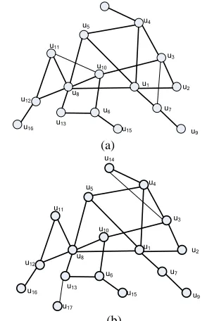
Example 1: Consider the two graphs in Fig. 2. We first compute their global node similarity matrix Sg. We construct a bipartite graph Gb with |V(G1)|+|V(G2)| nodes, and for any u ∈ V(G1) and v ∈ V(G2), we add an edge (u,v) ∈ E(Gb) with weight Sg[u,v].
u1 u2
u11
u10
u9
u8
u7
u6
u5 u4
u3
u16 u15
u14
u13
u12
(a)
u1 u2
u11
u10
u9
u8
u7
u6
u5 u4
u3
u16 u15
u14
u13
u12
u17
[image:4.612.341.488.430.658.2](b)
Figure 2: Two Graphs. (A) Graph G1, (B) Graph G2
(u11,v3), (u12,v6), (u13,v14), (u14,v15), (u15,v16), (u16,v9)}. In this way, the number of matched edges is 10, which is far away from the optimal solution mcs(G1, G2), 21 (bold edges in Fig. 2). Comparing to the optimal solution, u3 is mismatched to v7 because they have a high global similarity, but obviously, the local structure near u3 and the local structure near v7 differ much.
Alternative global node similarity measures:
Besides the global node similarity based on eigende composition, there are other global similarity measures based on the node importance in the graph in the literature, such as Katz score [9] and random walk with restart (RWR) [3]. A Katz score is a weighted count of the number of walks originating (or terminating) at a given node. The walks are weighted inversely by their length so that long and highly indirect walks count less, while short and direct walks count larger. The Katz score is given by the formula r = (I− bA)−1bAu, where r
is the N × 1 column vector containing Katz score for each node, I is the N×N identity matrix, u is a N×1 column vector with all entries equal to 1, and b
∈ (0, 1) is the attenuation factor, which is 1/(d+1) by default in [4],where d is the maximum degree of the graph. The extent to which the weights attenuate with length is controlled by b. The RWR score is given by the formula r= (1−c)(I −cW)−1u, where W is a transmit matrix where W(i, j ) = A(i, j)∑i A(i,
j), and c ∈[0, 1] is the positive probability, which means a surfer at a node will jump to a random node with probability 1 − c. Under this random walk, the importance of a node v is the expected sum of the importance of all the nodes u that link to v. For two nodes, u in graph G1 and v in graph G2, they are considered highly similar if both have a high Katz/RWR score. The similarity matrix of two graphs becomes S’g = r1r2 T. In Sect. 8, we report the effectiveness of these global node similarity measures.
The global node similarity gives a node similarity measure from the global point of view. However, when G1 and G2 are not sufficiently similar to each other, using global node similarity only is not sufficient to get a good matching because the global node similarity does not consider the local information for nodes in two graphs. We need a local node similarity.
Local node similarity: For any node v in graph G and k≥0, we define the k-neighborhood of v,N vk( ), as the set of nodes in V(G) such that v/ ∈
( )
k
N v and for any u ∈N vk( ), the shortest distance
from v to u is no more than k. The shortest distance is defined as the number of edges in the shortest path from v to u. The k-neighborhood subgraph of v
in G, denoted as Gvk, is defined as the induced subgraph over N vk( ) ∪{v} in G. For two nodes u
∈ V(G1) and v ∈ V(G2), we measure their local node similarity by comparing the k-neighborhood subgraphs of them. Suppose d(u) and d(v) are the degrees of node u and v in G1 and G2, respectively, and suppose d1,1, d1,2,... is the degree sequence of node set N (u)k in
k u
G sorted in non-increasing order, and d2,1, d2,2,... is the degree sequence of node set
( )
k
N v in k
v
G sorted in non-increasing order. Let nmin = min{| N uk( ) |, | N vk( ) |}.We define a
|V(G1)|×|V(G2)| local node similarity matrix Sl as follows.
2 min
( 1 ( , ))
[ , ]
(| ( ) | | ( ) |)(| ( ) | | ( ) |)
l k k k k
u u v v
n D u v
S u v
V G E G V G E G
+ + =
+ + (4)
min
1, 2, 1
min{ ( ), ( )} min{ , }
[ , ]
2 n
i i
i
d u d v d d D u v = +
∑
= (5)Here, D(u,v) consists of two parts. The first part min{d(u), d(v)} is the ideal contribution of edges when matching u with v, and the second part
min
1, 2, 1min{ , }
n
i i
i= d d
∑
is the ideal contribution of edges when matching nodes in N uk( )with nodes in N vk( ).We show that Sl has the following properties. 1. 0 < Sl [u,v]≤ 1.
2.
2
(| ( ( , )) | | ( ( , )) |)
[ , ]
(| ( ) | | ( ) |)(| ( ) | | ( ) |)
k k k k
u v u v
l k k k k
u u v v
V mcs G G E mcs G G
S u v
V G E G V G E G
+ =
+ +
3. If k u G and k
v
G are isomorphic, and u matches v in the optimal matching of k
u G and k
v
G , then Sl [u,v]= 1.
4. If k u
G is subgraph isomorphic to k v
G , and u matches v in the optimal matching of k
u G and
k v
G , we have Sl [u,v]= | (| ( ) |) | | (| ( ) |) | k k u u k k v v V G E G V G E G
+ +
For (1), it is obvious that Sl [u,v] >0 holds, because both (nmin+1+D(u,v))2>0 and
(| ( k) | | ( k) |)(| ( k) | | ( k) |)
u u v v
V G + E G V G + E G > 0. Sl [u,v]≤1
can be showed as follows. Since min{d(u), d(v)}≤ d(u) and min{d1,i , d2,i } ≤ d1,i ,
min 1, 1 ( ) [ , ] 2 n i i d u d
D u v≤ +∑= =|E(Guk )|. Similarly, D(u,v) ≤
|E( k v
G )|. By combining such two inequations with the fact that nmin + 1 ≤|V( k
u
G )| and nmin + 1 ≤
|V( k v
G )|,we have Sl [u,v]≤ 1. For (2), since the node number of either k
u
G or k
v
G appearing inmcs can never exceed the minimum node number of k
u G
and k v
G , |V(mcs( k u
G , k
v
G ))|≤n min + 1. Also, D(u,v) is known to be an upper bound of |E(mcs( k
u
G , k
ISSN: 1992-8645 www.jatit.org E-ISSN: 1817-3195
property (2) as an accurate similarity of two nodes based on their MCS. For (3), this can be obtained based on the illustration of the first property, since when they are isomorphism, we have nmin + 1
=|V( k
u
G )|=|V( k
v
G )| and D(u,v)
=
min 1, 1
( )
2 n
i i
d u +
∑
= d=|E( k u
G )|, while leads to St[u,v]=
| ( ) | | ( ) | | ( ) | | ( ) | k k u u k k v v
V G E G
V G E G
+
+ . Note that our local similarity [Eq.
(4)] is different from the vector-based node signature [5] which deals with edge weights. For an undirected and unweighted graph, the edge weights for all its incident edges are 1. This means that the node signature in [5] is merely its node degree, and measuring the similarity of two nodes by their degrees is not sufficient, because there might be many pairs of nodes, which share the same degree but are with different structures. In our local similarity measure, we do not only consider the degrees of two nodes but also consider their k-neighborhoods. [15] is one specific case of our local similarity when k = 0 for undirected and unweighted graphs.
Example 2 Reconsider the two graphs in Fig. 2. Let k = 2. The similarity matrix S of G1 and G2 is shown in Fig. 3b.We construct a bipartite graph Gb with |V(G1)|+|V(G2)| nodes, and for any u ∈
V(G1) and v ∈ V(G2), we add an edge (u,v) ∈
E(Gb) with weight S[u,v] (instead of Sg[u,v]). We compute the maximum weighted bipartite matching of Gb and get the matching M ={(u1,v1), (u2,v2), (u3,v3), (u4,v4), (u5,v5), (u6,v12), (u7,v13), (u8,v8), (u9,v17), (u10,v10), (u11,v14), (u12,v6), (u13,v11), (u14,v15), (u15, v9), (u16,v16)}. The number of matched edges is 13, which is better than 10 when only using the global similarity. But it is still much less than the optimal solution, 21.
4.2 A Problematic Approach To Compute M
Using S:
[2] computes a matching M by applying the Hungarian algorithm to the node similarity matrix, which can be with S we newly proposed or Sg given in [12]. Using all the similar node pairs computed, a matching M can be found. In order to compute a matching, [2] constructs a bipartite graph Gb that includes |V(G1)|+|V(G2)| nodes. For any node u ∈ V(G1) and node v ∈ V(G2), an edge (u,v) is added to Gb with weight S[u,v] (or Sg[u,v]). The maximum weighted bipartite matching of Gb leads to a matching M of graphs G1 and G2. Such an approach has two drawbacks.
– Similarity optimality does not mean matched edge optimality, while our aim is to maximize the number of matched edges in two graphs. It is
possible that two nodes are very similar in terms of S (or Sg) but the two nodes do not have many incident edges that help to increase the number of matched edges. As an example, suppose node u1 ∈
V(G1) and node v1 ∈ V(G2) all have degree 1, and S[u1,v1]= 1.0, and node u2 ∈ V(G1) and node v2
∈ V(G2) all have degree 10, and S[u2,v2]= 0.9. Suppose (u1,v1) is in conflict with (u2,v2) when computing the maximum weighted bipartite matching. In constructing the initial matching, the algorithm may give up (u2,v2) because it has a lower similarity. But obviously, giving up (u1,v1) is a better solution because (u2,v2) can contribute a larger number of matched edges, although u2 and v2 have lower node similarity.
– This approach only considers the matching of individual nodes in two graphs, and does not consider whether the nodes around them can be well matched when it matches two nodes. In other words, matching u ∈ V(G1) with v ∈ V(G2) does not consider whether the nodes around u and v can be matched using the maximum weighted bipartite matching. When the nodes around u and v are mismatched, even if u and v are similar, it can significantly affect the quality of the final matching M.
4.3 Anchor Selection And Expansion
In our approach, we solve the two drawbacks as follows. Instead of matching all the nodes, we first match some important nodes as anchors. Every two anchors matched have high similarity and large degrees, and can contribute a large number of matched edges. Then, we expand from the anchors to match the other nodes using the local similarity Sl as the measure. Thus, our solution consists of two steps, namely anchor selection and anchor expansion.
The anchors selected play two important roles in matching construction. (1) The matching anchors contribute a large number of edges to the matching M. (2) The anchors are the references to start with when matching the other nodes. For two nodes u ∈
V(G1) and v ∈ V(G2), we select (u,v) as matched anchors, if they satisfy the following two conditions.
(1) min{d(u), d(v)}≥ δ,where δ is the larger average degree of the two graphs, that is,
δ = max 1 2
1 2
2 | ( ) | 2 | ( ) |
,
| ( ) | | ( ) |
E G E G
V G V G
× ×
.
The algorithm for anchor selection is shown in Algorithm 2. Given two graphs G1 and G2, it outputs a list of anchor pairs, denoted asA. In the algorithm,S1 and S2 denote the sets of matched nodes in V(G1) and V(G2), respectively.
Algorithm 2 anchor-selection (G1, G2) Require: two graphs G1 and G2; Ensure: a list of matched anchor pairs A; 1: compute the similarity matrix S; 2: A ← ∅; S1 ← ∅; S2 ← ∅;
3: for all u ∈ V(G1) and v ∈ V(G2) in decreasing order of their similarity S[u,v] do
4: if S[u,v]≥τ and min{d(u), d(v)}≥δ and u / ∈ S1 and v/ ∈ S2 then
5: A ← A ∪{(u,v)}; S1 ← S1 ∪{u}; S2 ← S2
∪{v}; 6: return A;
Line 1 computes the similarity matrix S [Eq. (2)]. Line 3 tries to match the pairs (u,v) for all u ∈
V(G1) and v ∈ V(G2) in the decreasing order of their similarity. In this way, the most similar pairs will have a large chance to be matched as the anchors. Line 4 selects the nodes that satisfy the two conditions for anchor selection that are not matched before. If the conditions in line 4 are all satisfied, we add the pair (u,v) into the list A and add the matched nodes u and v into S1 and S2, respectively in line 5. After checking all pairs, line 6 returns A as the anchor pairs.
Example 3 Consider the two graphs in Fig. 2. Suppose τ = 0.94, using Algorithm 2, we can get the set of anchor pairs to be A ={(u1,v1), (u8,v8)}. Obviously, the correct matching of the two pairs is very important in the final matching of G1 and G2. For the pair (u9, v17), although it satisfies the similarity constraint, it destroys the degree constraint. Obviously, expanding from the pair (u9,v17) to match other pairs is a bad choice.
Theorem 1 The time complexity of Algorithm 2 is O(|V(G1)|2 · (|V(G1)|+|E(G1)|) + |V(G2)|2 ·(|V(G2)|+|E(G2)|)).
Proof 1 Algorithm 2 is to select anchors. Computing the global node similarity matrix needs O(|V (G1)|3+|V(G2)|3) time, and computing the local node similarity matrix needs O(|V(G1)|2
·|E(G1)|+|V(G2)|2 ·|E(G2)|) time. In lines 3-5,
sorting all pairs needs O(|V(G1)|·|V(G2)|·(log(|V(G1)|) + log(|V(G2)|)))
time. Hence, the overall time complexity of Algorithm 2 is O(|V(G1)|2 · (|V(G1)|+|E(G1)|)
+|V(G2)|2 · (|V(G2)|+|E(G2)|)).
We illustrate the anchor expansion algorithm (Algorithm 3) to obtain a matching M. Let A be the anchor pairs (u,v) selected already. Initially, M = A.
Let N(u) and N(v) denote the immediate neighbors of u and v in graphs G1 and G2, respectively. For every matched pair (u,v) in the initial M, we put all (N(u)× N(v)) pairs in a queue Q, where Q is the set of candidate matching pairs sorted in decreasing order of their local similarity. In an iterative manner, we remove the pair (u,v) with the largest local similarity Sl [u,v] [Eq. (4)] from Q. If both u and v have not been matched before, we add (u,v) to M and put their all (N(u) × N(v)) immediate neighbor pairs into Q for further consideration. We repeat it until Q =∅.
Algorithm 3 anchor-expansion (G1, G2, A) Require: two graphs, G1 and G2, and the anchor pairs A;
Ensure: a graph matching M; 1: M ← A; Q ← ∅; S1 ← ∅; S2 ← ∅; 2: for all (u,v) ∈ A do
3: S1 ← S1 ∪{u}; S2 ← S2 ∪{v}; Q ← Q ∪
(N(u) × N(v)); 4: while Q≠∅ do
5: remove (u,v) from Q with the largest similarity Sl [u,v];
6: if u
∉
S1 and v∉
S2 then7: M ← M ∪{(u,v)}; S1 ← S1 ∪{u}; S2 ← S2
∪{v}; Q ←Q ∪ (N(u) × N(v)); 8: return M;
The example of anchor expansion is given below.
Example 4 Given the two graphs in Fig. 2.After we get the set of anchor pairs A ={(u1,v1), (u8,v8)}. Using Algorithm 3, we can construct our matching M ={(u1,v1), (u2,v7), (u3,v3), (u4,v4), (u5,v5), (u6,v6), (u7,v2), (u8,v8), (u9,v9), (u10,v10), (u11,v13), (u12,v12), (u13,v11), (u14,v14), (u15,v15), (u16,v16)}. The number of matched edges is 18.
Theorem 2 The time complexity of Algorithm 3 is O(|V(G1)|·|V(G2)|· min{|V(G1)|, |V(G2)|}).
Proof 2 Algorithm 3 is to expand from the anchors selected. The dominant part of the time complexity is line 5 and line 7. For line 5, there are at most |V(G1)|·|V(G2)| pairs, and for each pair, it needs O(|V(G1)|·|V(G2)|) to obtain the one with the largest similarity. For line 7, there are at most min{|V(G1)|, |V(G2)|} matched pairs, and for each pair, it needs O(|V(G1)|·|V(G2)|) to compute the cartesian product. Therefore, the overall time complexity is O(|V(G1)|·|V(G2)|· min{|V(G1)|, |V(G2)|}).
4.4 Discussion On Τ For Anchor Selection
ISSN: 1992-8645 www.jatit.org E-ISSN: 1817-3195
factor for the matching quality. It should be neither too large nor too small. When τ is too large, very few nodes will be selected as anchors, which lead to more nodes to be mismatched in anchor-expansion. The reason is that anchor-expansion is designed as a greedy algorithm and can only achieve local optimum. For a node in a graph, the more steps it needs to be expanded from an anchor, the higher the probability to be mismatched. When τ is too small, a large number of anchor pairs may be selected, and many mismatched anchors are thus involved. Expanding from these mismatched anchors will hardly lead to a good matching result. We explain it using an example.
Example 5 Reconsider Example 3 in Sect. 5. Suppose we set τ to a very small value, that is, τ = 0.78, for graphs in Fig. 2. A large set of anchor pairs is obtained: A = {(u1,v1), (u4,v4), (u5,v5), (u6,v12), (u7,v13), (u8,v8), (u10,v10), (u12,v6)}. If we then run anchor-expansion based on this A, we obtain the matching result M ={(u1,v1), (u2,v2), (u3,v3), (u4,v4), (u5,v5), (u7,v13), (u8,v8), (u9,v17), (u10,v10), (u12,v6), (u13,v11), (u14, v14), (u15,v16), (u16,v15)}. The number of matched edges is 16, which is not as good as the matching result in Example 4 (The number of matched edges is 18). This is because a small τ makes several mismatched anchor pairs {(u6,v12), (u7,v13), (u12,v6)} included in A. Expanding from such mismatched anchor pairs will make the matching result ineffective. On the other hand, suppose we set τ to a very high value, that is, τ = 0.98. No anchor pair will be selected. Under such circumstances, one node will be randomly selected from each graph to form an anchor pair, and expanding from such a random anchor pair is unlikely to lead to a good matching.
It is difficult to determine an appropriate τ for graph matching, because τ is not related to graph sizes or degree distributions. One attempt we made is to collect some statistics from the similarity matrix S to see whether there is certain relationship between S and τ . First, we set τ to be a small value 0.5 and select an initial list of anchor pairs AI using Algorithm 2. Then, we divide the interval [0.5, 1] to disjoint small intervals (bins) with equal length l , and count the number of anchor pairs (u,v) in a bin if S[u,v] is in its interval. We take τ to be used as the middle value of the bin, which has the smallest number of anchor pairs. This means that we choose a significant gap as threshold τ to be used. However, in our extensive experimental studies, the matching results obtained by using such a τ are not necessarily guaranteed to be good. In order to ensure a good initial graph matching, we select the
best τ by exploring all τ with every step of l in [0.5, 1], for example, 0.5, 0.5 + l, 0.5 + 2l,..., and choosing the τ value that results in the best graph matching M (the output of anchor-expansion). Such process is shown in Algorithm 4.With Algorithm 4, Algorithm 1 can be modified by replacing line (1– 2) with construct-opt(G1, G2). In order to further reduce the cost, as a heuristics, we adopt a hill climbing method. We set the default value of τ = 0.9, and set the step length l to 0.02, and choose the direction by comparing the matching result for τ = 0.9−l and τ = 0.9+l to start climbing. The climbing will stop when the current value is less than the best value we have obtained or the value of τ is out of range [0.5, 1]. Such a hill climbing method stops within several steps and achieves good results, as can be seen in our testing.
Algorithm 4 construct-opt (G1, G2) Require: two graphs, G1 and G2;
Ensure: a graph matching between G1 and G2; 1: τ ← 0.5; Mopt ← ∅;
2: AI ←anchor-selection (G1, G2); {Algorithm 2}
3: for all τi = 0.5 + i × l such that τi ∈[0.5, 1] do
4: A ←{(u,v)|(u,v) ∈ AI, S[u,v]≥τi };
5: M ← anchor-expansion (G1, G2,A); {Algorithm 3}
6: if score(M)> score(Mopt ) then 7: Mopt ← M;
8: return Mopt ;
Theorem 3 The time complexity of Algorithm 4 is O(|V(G1)|2 · (|V(G1)|+|E(G1)|) +|V(G2)|2 ·
(|V(G2)|+|E(G2)|)).
Proof 3 The dominant part of Algorithm 4 is line 2 and lines 3–7. For line 2, the time complexity of anchor-selection is shown to be O( |V (G1)|2·(|V(G1)|+|E(G1)|)+ |V(G2)|2 ·(|V(G2)|+ |E(G2)|)) in Theorem1. For lines 3–7, since the time complexity of anchor-expansion is shown to be O( |V(G1)|·|V(G2)|· min {|V(G1)|, |V(G2)|}) in Theorem 2, the total complexity of lines 3–7 is O(c·|V(G1)|·|V(G2)|· min {|V(G1)|,|V(G2)|}) where c is the steps that we need in the loop. Usually, c = 0.5/l is a small constant for a given l . So the total complexity of Algorithm 4 is O(|V(G1)|2 · (|V(G1)|+|E(G1)|) + |V(G2)|2 ·(|V(G2)|+|E(G2)|)).
5 CONCLUSION AND FUTURE WORK
selection is the dominant factor and anchor-expansion can be done very quickly in practice compared to anchor-selection. Some results are shown that the time of anchor-expansion means the total expansion time including the τ selection.
REFERENCES:
[1] T. Plantenga, “Inexact subgraph isomorphism in MapReduce”, Journal of Parallel and Distributed Computing, Vol. 73, No. 2, 2013, pp. 164-175.
[2] F. Kuhn, and M. Mastrolilli, “Vertex cover in graphs with locally few colors”, Information and Computation, Vol. 222, No. 0, 2013, pp. 265-277.
[3] A. Egozi, Y. Keller, and H. Guterman, “A Probabilistic Approach to Spectral Graph Matching”, Pattern Analysis and Machine Intelligence, IEEE Transactions on, Vol. 35, No. 1, 2013, pp. 18-27.
[4] T. S. Caetano, J. J. McAuley, C. Li et al., “Learning Graph Matching”, Pattern Analysis and Machine Intelligence, IEEE Transactions on, Vol. 31, No. 6, 2009, pp. 1048-1058
[5] L. Zhi-Yong, Q. Hong, and X. Lei, “An Extended Path Following Algorithm for Graph-Matching Problem”, Pattern Analysis and Machine Intelligence, IEEE Transactions on,
Vol. 34, No. 7, 2012, pp. 1451-1456.
[6] H. Xiong, D. Xiong, Q. Zhu et al., “A Structured Learning-Based Graph Matching Method For Tracking Dynamic Multiple Objects”, Circuits and Systems for Video Technology, IEEE Transactions on, Vol. PP, No. 99, 2012, pp. 1-1.
[7] P. Doshi, R. Kolli, and C. Thomas, “Inexact matching of ontology graphs using expectation-maximization”, Web Semantics: Science, Services and Agents on the World Wide Web,
Vol. 7, No. 2, 2009, pp. 90-106.
[8] T. Ersal, H. K. Fathy, and J. L. Stein, “Structural simplification of modular bond-graph models based on junction inactivity”,
Simulation Modelling Practice and Theory, Vol. 17, No. 1, 2009, pp. 175-196.
[9] Z. Nutov, “Survivable network activation problems”, Theoretical Computer Science, No. 0, 2012.
[10] S. Kpodjedo, P. Galinier, and G. Antoniol, “Using local similarity measures to efficiently address approximate graph matching”, Discrete Applied Mathematics, No. 0, 2012.
[11] L. Sun, and T. Chen, “Comparing the Zagreb indices for graphs with small difference between the maximum and minimum degrees”,
Discrete Applied Mathematics, Vol. 157, No. 7, 2009, pp. 1650-1654.
[12] J.-K. Hao, and Q. Wu, “ Improving the extraction and expansion method for large graph coloring ” , Discrete Applied Mathematics, Vol. 160, No. 16, 2012, pp. 2397-2407.
[13] A. Bhattacharjee, and H. Jamil, “WSM: a novel algorithm for subgraph matching in large weighted graphs”, Journal of Intelligent Information Systems, Vol. 38, No. 3, 2012, pp. 767-784.
[14] M. Zaslavskiy, F. Bach, and J. P. Vert, “A Path Following Algorithm for the Graph Matching Problem”, Pattern Analysis and Machine Intelligence, IEEE Transactions on, Vol. 31, No. 12, 2009, pp. 2227-2242.
[15] L. Zhu, W. Keong Ng, and J. Cheng, “Structure and attribute index for approximate graph matching in large graphs”, Information Systems,
Vol. 36, No. 6, 2011, pp. 958-972.
[16] T. Yamada, and T. Shoudai, “Efficient Pattern Matching on Graph Patterns of Bounded Treewidth”, Electronic Notes in Discrete Mathematics, Vol. 37, No. 0, 2011, pp. 117-122.
[17] J. Lebrun, P.-H. Gosselin, and S. Philipp-Foliguet, “Inexact graph matching based on kernels for object retrieval in image databases”,
Image and Vision Computing, Vol. 29, No. 11, 2011, pp. 716-729.
[18] C. Jiefeng, J. X. Yu, and P. S. Yu, “Graph Pattern Matching: A Join/Semijoin Approach”,
Knowledge and Data Engineering, IEEE Transactions on, Vol. 23, No. 7, 2011, pp. 1006-1021.
[19] R. Erman, M. Krnc et al., “Improved induced matchings in sparse graphs”, Discrete Applied Mathematics, Vol. 158, No. 18, 2011, pp. 1994-2003.
[20] D. Emms, R. C. Wilson, and E. R. Hancock, "Graph matching using the interference of discrete-time quantum walks," 7th IAPR-TC15 Workshop on Graph-based Representations (GbR 2007), 2009, pp. 934-949.