Abstract—Current study of myocardial motion on echocardiography mainly focused on the improvement of the motion accuracy, whereas the quantification of myocardial motion is a key task for motion analysis and interpretation by cardiologist. Therefore, we proposed a features extraction method to provide information on the segmental boundary profile of myocardial motion. Once the optical flow of two consecutive frames is computed, then we take out only flow field on the inner boundary instead of the whole myocardium. The inner boundary is detected using Canny operator and centroidal based searching method; and then applying B-spline and statistical outliers remover to smoothen the boundary. The complete profile consists of displacement and radial direction of every segment at any frame from end-diastole to end-systole. The validation is performed by comparing the computed profile and the manual analysis by cardiologist. In conclusion, this profile is in agreement and has capability to be used to detect an abnormal segment more accurately.
Index Terms—2-dimensional echocardiography, segmental myocardial motion, localize abnormalities, optical flow.
I. INTRODUCTION
[image:1.612.319.537.187.257.2]Anatomically, the blood supply for every part of the heart is provided by coronary arteries. Fig. 1 shows an illustration of the heart and coronary arteries, namely right coronary artery (RCA), left coronary artery (LCA), left circumflex artery (LCx) and left anterior descending artery (LAD) artery. A coronary artery supplies blood to one segment or more of the heart as tabulated in
Table 1. When the blood supply to the heart is interrupted, heart attack can occur.
Fig. 1. Illustration of heart and coronary arteries [1]
Manuscript received March 3, 2010. This work was supported by the Universiti Kebangsaan Malaysia under grant UKM-GUP-TKP-08-24-080.
Slamet Riyadi, Mohd Marzuki Mustafa and Aini Hussain are with the Department of Electrical, Electronic and Systems Engineering, Faculty of Engineering and Built Environment, Universiti Kebangsaan Malaysia, Bangi 43600 Malaysia (email: riyadi, marzuki, [email protected]).
[image:1.612.122.248.534.635.2]Oteh Maskon and Ika Faizura Mohd Noh are with Cardiac Care Unit, Medical Center, Universiti Kebangsaan Malaysia, Kuala Lumpur 56000 Malaysia.
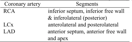
Table 1. Coronary arteries and their associate segments [2] Coronary artery Segments
RCA inferior septum, inferior free wall & inferolateral (posterior) LCx anterolateral and posterolateral LAD anterior septum, anterior free wall
and apex
Heart attack, which is a major cause of death all over the world, is commonly affected by coronary heart disease. It can be detected early by monitoring left ventricular (LV) motion abnormality. This is the reason why the study and analysis of LV motion is very important; hence it has been an active research in the past decade.
Physicians estimate LV motion by utilizing magnetic resonance imaging (MRI), single photon emission computed tomography (SPECT) or ultrasound. LV motion analysis using MRI and SPECT has successful stories as reported in [3][4][5], since these modalities produce relatively noise-free images. However, they have several problems along with their portability, invasive and radiation issues. Ultrasound modality has a great potential to overcome these issues. The promising prospect attracts many researchers to investigate using echocardiography. Boukerroui et al
proposed a block matching approach to estimate cardiac velocity on B-mode ultrasound images. They combined two existing techniques (similarity measurement by Cohen-Dinstein and Singh block matching) to compute velocities only at contour points. The proposed approach however has a large error after one cardiac cycle due to error propagation from frame to frame [6]. Other motion estimation which can measure myocardial border segmentation was proposed using deformation model on 3D echocardiography [7]. In certain methods of myocardial border detection, errors are introduced when the motion is parallel to border [8]. Ledesma-Carbayo et al proposed a spatio-temporal non-rigid registration to estimate myocardial motion for 2D ultrasound cardiac motion estimation. This paper extensively describes a parametric spatio-temporal deformation model and global optimization using multiresolution approach. The results obtained with real data, promises a great potential to provide myocardial motion assessment for echocardiography. An extensive research should be conducted to derive a quantitative evaluation to localize ischemic segment [8]. Other popular technique for cardiac motion estimation is to use optical flow method. Mikic et al used active contours guided by optical flow to perform segmentation and tracking in echocardiography, while Veronesi et al, Becciu et al and Duan et al utilized
Segmental Boundary Profile of Myocardial
Motion to Localize Cardiac Abnormalities
optical flow on real-time 3D echocardiography [9][10][11][12]. Riyadi et al enhanced optical flow field of left ventricular motion on 2D echocardiography using quasi Gaussian DCT filter [13]. Various modifications on optical flow method indicate that this approach has the prospective to be utilized in cardiac motion analysis.
According to our review, current research mainly focused on how to improve the accuracy of cardiac motion estimation, since it is quite difficult to detect the myocardial motion using ultrasound modality. The difficulties may be caused by the presence of speckle noise which is introduced by the limitation of ultrasound modality. Additionally, improper image acquisition also makes harder to detect the cardiac motion. On the other hand, quantification of computed motion will be very useful for physician to interpret the cardiac motion and hence support the clinical decision. Therefore, in this paper we propose profile extraction of computed optical flow, instead of the motion estimation itself. Segmental profile will cover from end-diastole to end-systole thus it can be utilized to localize the presence of suspected abnormal segment and coronary artery.
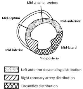
[image:2.612.331.531.194.317.2]II. UNDERSTANDING LEFT VENTRICULAR MOTION The Cardiac Imaging Committee of the Council on Clinical Cardiology of the America Heart Association has released a standardized myocardial segmentation and nomenclature for tomography imaging of the heart. It includes four standard views for echocardiographic image collection from patient, i.e. parasternal long axes (PLAX), parasternal short axis (PSAX), apical four chambers (A4C) and apical two chambers (A2C). In this paper, the evaluation of myocardial movement is focused only on the PSAX view as shown in Fig. 2. The cavity of left ventricular appears in a center surrounded by six myocardial segments. The normal cardiac appearance is indicated by a uniform displacement of myocardial segments. They move in radial forward and backward directions with respect to the center of cavity, which describe the profile of systole and diastole of a cardiac. In one full cycle, the cavity size will shrink progressively during systole, and followed by a brief instance of diastole that recovers the cavity [14].
Fig. 2. PSAX view of echocardiography image and its segments [15]
III. ENHANCED OPTICAL FLOW COMPUTATION Riyadi et al. introduced a filtering approach, called quasi Gaussian DCT (QGDCT) filter, which is used to suppress speckle noise of ultrasound images and enhance the computed optical flow field [13]. Considering the 8th cosine
basis of 1D DCT function as shown in Fig. 3, a quasi Gaussian kernel model is constructed by removing negative coefficients from the function Fig. 3. It can be seen that the model is similar to the natural discrete Gaussian kernel without the even term coefficients. The 2D QGDCT kernel is obtained by similar steps applied on the down-right function of 2D DCT basis in Fig. 3.
(a)
(b) (c)
Fig. 3 (a) The selected 8th 1D DCT function, (b) a 1D
quasi-Gaussian model, and (c) 2D cosine basis function Computation of optical flow assumes that the intensity of the object remains constant, which is represented by the intensity constraint equation
I(x, y, t) = I(x+δx, y+δy, t+δt) (1)
Within small values of δx, δy and δt, the intensity constraint can be represented using the 1st order Taylor series expansion
shown below, t t I y y I x x I t y x I t t y y x x
I δ δ δ δ δ δ
∂ ∂ + ∂ ∂ + ∂ ∂ + = + + + , , ) (, ,) ( (2)
Simplifying equation (1) and (2), the basic constraint of the optical flow equation can be expressed as
0 = +
+I dy I dt
dx
Ix y t , or Ixu+Iyv+It =0 (3) The Horn-Schunck’s method, includes global smoothness error (ES) and brightness constancy error (EC) defined as [17]
2 2 2 2 dxdy y v x v y u x u
ES
∫∫
⎟⎟⎠ ⎞ ⎜ ⎜ ⎝ ⎛ ⎟⎟ ⎠ ⎞ ⎜⎜ ⎝ ⎛ ∂ ∂ + ⎟ ⎠ ⎞ ⎜ ⎝ ⎛ ∂ ∂ + ⎟⎟ ⎠ ⎞ ⎜⎜ ⎝ ⎛ ∂ ∂ + ⎟ ⎠ ⎞ ⎜ ⎝ ⎛ ∂ ∂ = (4) ) (u x v y t2dxdy
EC=
∫∫
∇ +∇ +∇ (5) Optical flow vector (u, v) is then computed using an iterative solution to minimize E = λEC + ES, where λ is a suitable weighting factor.IV. SEGMENTAL PROFILE EXTRACTION
[image:2.612.117.259.530.682.2]MN
j i v j i u D
M i
N j S
∑ ∑= = +
= 1 1 (, )2 (, )2 (5) This displacement indicates only the magnitude of myocardial motion. Since the normal myocardial moves to the center of cavity, it is important to provide radial direction of the motion as illustrated in Fig. 4. The segmental radial direction is the average of radial directions for single pixel in a myocardial segment.
MN j i
M i
N j S
∑ ∑= = = 1 1α(, )
α (6)
Fig. 4. Illustration of radial direction of optical flow with respect to the center of cavity
In the method described earlier, both displacement and radial direction profiles were computed by considering all myocardial motion fields. However, the ultrasound modality produces random speckle images that may influence the computation of motion field on the myocardium area and potential to introduce errors. Hence, to provide more accurate myocardial profile, we only use the motion values on the inner myocardium boundary instead of all pixel motions on myocardium.
Inner boundary of myocardium, or known as endocardium, is initially processed by Canny edge detection operator. Canny operator produces a global edge of whole cardiac image. The inner boundary is then searched from the cavity center. The Canny edge that has the nearest distance from the center is retained as the inner boundary. Since the initial boundary is discontinuous and not smooth, a numerical B-spline function and statistical outliers remover are applied to obtain a continuous and smooth boundary.
V. RESULT AND DISCUSSION
A. Computed Optical Flow
In this paper, we use clinical echocardiography data which are recorded previously by physician. These data are acquired on PSAX view from a healthy volunteer and a patient using a Siemens Acuson Sequoia scanner. A cardiologist has manually performed the qualitative segmental analysis by scoring each segment according to a standardized codes, i.e 1=normal, 2=hypokinetic and 3=akinetic [18]. Fig. 5 shows four frames of ten consecutive sequences that describe normal cardiac motion from end-diastole to end-systole.
(a) (b)
[image:3.612.312.525.45.222.2](c) (d)
Fig. 5. Four frames of normal cardiac motion from end-diastole to end-systole: (a) 1st (b) 4th (c) 7th and (d) 10th
frame
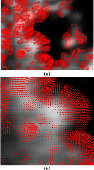
Fig. 6(a) shows the computed optical flow for myocardial motion of two consecutive images of 4th and 5th frame. The
optical flow arrows, which are superimposed on the smoothed image of 4th frame, represent the displacement of
the pixels and their directions. Fig. 6(b) shows the zoomed appearance of optical flow arrows on the mid anterior segment (down right of the LV). These figures show that the enhanced optical flow technique gives a more correct direction of myocardial motion compared to the computed flow fields which were smoothed by mean, median or Frost filter, as detailed in [13]. The correct and smooth arrows were obtained on the inner myocardium boundary as shown evidently in Fig 6(b). However, we found errors on the
(a)
(b)
Fig. 6. (a) Computed optical flow of two consecutive images, 4th and 5th frame; (b) zoom-in mid inferior segment
Optical flow arrow
o
Center of cavity
α = Radial direction with respect to the center of cavity
o
[image:3.612.74.251.156.287.2] [image:3.612.355.509.423.700.2]direction of flow field inside the myocardium, which is mainly due to the presence of random speckle noise. Furthermore, in order to quantify accurately the myocardial profile, we need only consider extracting the profile from the computed motion on the inner boundary, instead of all flow fields on the myocardium.
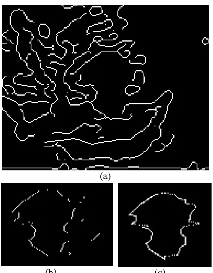
To detect the inner boundary, firstly we compute global edge of cardiac image using Canny operator as shown in Fig. 7(a). Using the computed Canny edge, we search the initial inner boundary as given in Fig. 7(b). Since the initial boundary is discontinuous, afterward a numerical B-spline function and statistical outliers removal are applied and obtain a smooth boundary in Fig. 7(c).
(a)
(b) (c)
Fig. 7. (a) Computed global Canny edge of 4th frame; (b)
Initial inner boundary and (c) final smoothed boundary
B. Segmental Boundary Profiles
Fig. 8(b) shows the myocardial boundary motion at 4th
frame for normal cardiac shown in Fig. 5 . This flow field is extracted by computing the mean of 5x5 neighbouring pixels along the boundary. By manual observation, it can be seen that the arrows agree with the manual scores which are previously determined by cardiologist as shown in Fig. 8(a). The endocardial obviously moves to the center of cavity with a relative constant displacement, as depicted in the distribution of boundary displacement and radial direction (Fig. 9(a) and (b)).
(a)
(b)
Fig. 8. (a) Cardiologist score for each segment (1=normal); (b) Extracted flow field on the inner boundary of 4th frame
0 0.5 1 1.5 2 2.5 3 3.5 0
50 100 150
Boundary displacement (pixels)
[image:4.612.356.508.46.319.2](a) (b)
Fig. 9 Distribution of (a) boundary displacement and (b) radial direction
The complete profile of segmental boundary on myocardial displacement and radial direction are depicted in Fig. 10(a) and Fig. 10(b), respectively. Fig. 10(a) shows that each segment moves with a uniform displacement within 0.8 – 1.5 pixels. Consistent with the manual inspection on 4th
frame, the complete segmental boundary profile of radial direction is in agreement with the cardiologist analysis. As shown in Fig. 10(b), radial direction of any segment is between 0 and 500 in every frame which indicates that the
segments move inward to the cavity center. However, the computed profile of a certain segment in a certain frame does not follow this trend. For example, mid anterior segment mostly does not move in 2nd frame and then move with a large
displacement in the next frame. This is expected since the displacement of a segment may vary from frame to frame.
1 1
1
[image:4.612.86.295.200.468.2] [image:4.612.315.530.368.481.2]1 2 3 4 5 6 7 8 9 0.2
0.4 0.6 0.8 1 1.2 1.4 1.6 1.8 2 2.2
Time (-th frame)
M
ea
n of
D
is
p
lac
em
ent
(pi
x
el
s
)
Mid anterior Mid anterior septum Mid septum Mid inferior Mid posterior Mid lateral
(a)
1 2 3 4 5 6 7 8 9
-200 -150 -100 -50 0 50 100 150
Time (-th frame)
M
ean of
R
a
di
a
l D
ir
ec
ti
on
(
deg
re
e)
Mid anterior Mid anterior septum Mid septum Mid inferior Mid posterior Mid lateral
[image:5.612.79.283.47.406.2](b)
Fig. 10 Segmental boundary profile of (a) displacement and (b) radial direction
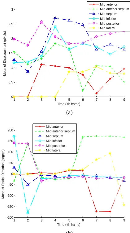
The following discussion is on the results of applying the proposed technique to an abnormal cardiac that has hypokinetic symptom on mid anterior, mid anterior septum and mid lateral. Fig. 11 shows four original images of the sequences frame from end-diastole to end-systole. This study has been analyzed manually by cardiologist by scoring each segment as depicted in Fig. 13(a).
(a) (b)
(c) (d)
Fig. 11. 1st , 4th, 7th and 10th frame of abnormal cardiac
[image:5.612.347.513.66.187.2]motion from end-diastole to end-systole.
Fig. 12. Manual scoring by cardiologist (1=normal, 2=hypokinetic
Three normal segments, i.e. mid septum, mid inferior and mid posterior, show relative constant displacement and correct radial direction as shown in Fig. 13(a) and (b). Mid anterior segment moves weakly along the frame at a correct direction, whereas the mid lateral has no displacement at the beginning motion of systole and then moves slightly in the rest of frames. Other interesting detail is the motion of mid anterior septum which moves with correct displacement and
1 2 3 4 5 6 7 8 9
0 0.5 1 1.5 2 2.5 3
Time (-th frame)
M
ea
n of
D
is
p
lac
em
ent
(pi
x
el
s
)
Mid anterior Mid anterior septum Mid septum Mid inferior Mid posterior Mid lateral
(a)
1 2 3 4 5 6 7 8 9
-200 -150 -100 -50 0 50 100 150 200
Time (-th frame)
M
e
an
of
R
adi
al
D
ir
ec
ti
on
(d
egr
ee)
Mid anterior Mid anterior septum Mid septum Mid inferior Mid posterior Mid lateral
(b)
Fig. 13. Segmental boundary profile of (a) displacement and (b) radial direction, from abnormal cardiac
2
2 1
1 1
[image:5.612.320.530.336.710.2] [image:5.612.83.298.530.711.2]direction at the beginning of systole. Afterwards, this segment moves with an opposite direction outward from center as shown in Fig. 14. This can be explained as the mid anterior septum actually moves with translation mode instead of contraction. This motion is not driven by the muscle of mid anterior septum but pulled by the motion of other segment. This is clinically known as pulling phenomenon. This fact indicates that there may be a problem with the LAD artery which supplies blood to the mid anterior septum segment.
Fig. 14 Pulling phenomenon on mid anterior septum
VI. CONCLUSION
In this paper, we have described a features extraction method to provide information on the segmental boundary profiles of myocardial motion from computed optical flow on echocardiography images. The inner boundary is selected because it produces more accurate profile than the myocardium due to the speckle noise problem. The complete profile describes the displacement and radial direction of each segment at any frame from end-diastole to end-systole. These profiles provide useful aid to cardiologist to observe and interpret the myocardial motion more accurately. Our preliminary result looks promising since the complete segmental profile is in agreement with the manual analysis by cardiologist and has ability to localize suspected abnormal segment. In future work, testing using a larger database will be performed to further validate the proposed method. Other parameters which represent the cardiac motion should also be determined to provide more complete and accurate diagnostic.
REFERENCES
[1] Texas Heart Institute, “Coronary artery spasm”, Heart Information Center [Online], August 2009, Available:
http://www.texasheartinstitute.org/HIC/Topics/Cond/CoronaryArtery Spasm.cfm
[2] C. M. Otto, “Ischemic cardiac disease”, Textbook of Clinical Echocardiogaphy, 3rd Ed., Pennsylvania: Elsevier Saunders, 2004, pp:196 – 226.
[3] H. Sundar, H. Litt and D. Shen, “Estimating myocardial motion by 4D image warping”, Pattern Recognition 42, 2009, pp. 2514–2526. [4] G. S. Lin, H. H. Hines, G. Grant, K. Taylor and C. Ryals, “Automated
quantification of myocardial ischemia and wall motion defects by use of cardiac SPECT polar mapping and 4-D surface rendering”, Journal of Nuclear Medicine Technology, Vol. 34 No. 1, 2006.
[5] A. Sunesiaputra, A. F. Frangi, T. A. M. Kaandorp, H. J. Lamb, J. J. Bax, J. H. C. Reiber and P. F. Lelieveldt, “Automated detection of regional wall motion abnormalities based on a statistical model applied
to multiscale short-axis cardiac MR images”, IEEE Transactions on Medical Imaging, Vol. 28 No. 4, April 2004, pp. 595 – 607. [6] D. Boukerroui, J. A. Noble, and M. Brady, “Velocity Estimation in
Ultrasound Images: A Block Matching Approach”, LNCS 2732, 2003, pp. 586–598.
[7] X. Papademetris, A. J. Sinusas, D. P. Dione and J. S. Duncan, “Estimation of 3D left ventricular deformation from
echocardiography”, Medical Image Analysis, Vol. 5, Issue 1, March 2001, pp. 17 – 28.
[8] M. J. Ledesma-Carbayo, J. Kybic, M. Desco, A. Santos, M. Suhling, P. Hunziker, and M. Unser, “Spatio-temporal nonrigid registration for ultrasound cardiac motion estimation”, IEEE Transactions on Medical Imaging, Vol. 24 No. 9, September 2005, pp. 1113 – 1126.
[9] I. Mikic, S. Krucinski, and J. D. Thomas, “Segmentation and tracking in echocardiographic sequences: Active contours guided optical flow estimates”, IEEE Transactions on Medical Imaging, Vol. 17 No. 2, April 1998, pp. 274 – 284.
[10] F. Veronesi, C. Corsi, E. G. Cainai, A. Sarti and C. Lamberti, “Tracking of left ventricular long axis from real-time
three-dimensional echocardiography using optical flow techniques”,
IEEE Transactions on Information Technology in Biomedicine, Vol. 10 No. 1, January 2006, pp. 174 – 181.
[11] A. Becciu, H. v. Assen, L. Florack, S. Kozerke, V. Roode, and B. M. t. H. Romeny, “A Multi-scale feature based optic flow method for 3D cardiac motion estimation”, LNCS 5567, 2009, pp. 588–599. [12] Q. Duan, E. D. Angelini, O. Gerard, K. D. Costa, J. W. Holmes, S.
Hommad, A. F. Laine, “Cardiac motion analysis based on optical flow on real-time three-dimensional ultrasound data”, Recent Advances in Diagnostic and Therapeutic Ultrasound Imaging for Medical Applications, 2006.
[13] S. Riyadi, M. M. Musatafa, A. Hussain, O. Maskon, and I. F. M. Noh, “Enhanced optical flow field of left ventricular motion using quasi Gaussian DCT filter”, to be appeared in Software Tools and Algorithms for Biological Systems, 2010.
[14] B. Anderson, “Chapter 2: The 2-dimensional echocardiographic examination”, Echocardiography: The Normal Examination of Echocardiographic Measurements, Blackwell Publishing, 2002. [15] H. Rimington and J. B. Chambers, “Echocardiography: A Practical
Guide”, 2nd Ed., London: Informa, 2007, ch. 2.
[16] S. Riyadi, M. M. Musatafa, A. Hussain, O. Maskon, and I. F. M. Noh, “Quasi-Gaussian DCT Filter for Speckle Reduction of Ultrasound Images”, LNCS 5857, 2009, pp. 136 - 147.
[17] Horn B.K.P and Schuck B.G (1981) Determining Optical Flow.
Artificial Intelligent, vol 9, pp 185-203.
[18] N. Schiller, P. Shah, and M. Crawford, “American Society of Echocardiography committee on standards, subcommittee on quantitation of two-dimensional echocardiograms: Recommendations for quantitation of the left ventricle by two-dimensional