Bayesian Inference for Spatial Beta Generalized Linear Mixed Models

Bayesian Inference for Spatial Beta Generalized Linear

Mixed Models

L. Kalhori Nadrabadi

1, 2

, and M. Mohhamadzadeh

*1

1 _{Department of Statistics, Faculty of Mathematical Sciences, Tarbiat Modares University, Tehran,}

Islamic Republic of Iran

2 _{Statistical Research and Training Center, Tehran, Islamic Republic of Iran}

Received: 18 October 2017 / Revised: 15 November 2017 / Accepted: 3 January 2018

Abstract

In some applications, the response variable assumes values in the unit interval. The

standard linear regression model is not appropriate for modelling this type of data

because the normality assumption is not met. Alternatively, the beta regression model

has been introduced to analyze such observations. A beta distribution represents a

flexible density family on (0, 1) interval that covers symmetric and skewed families. In

this paper, a beta generalized linear mixed model with spatial random effect is proposed

emphasizing on small values of the spatial range parameter and small sample sizes.

Then some models with both fixed and varying precision parameter and different

combinations of priors and sample sizes are discussed. Next, the Bayesian estimation of

the model parameters is evaluated in an intensive simulation study. Selected priors

improved the Bayesian estimation of the parameters, especially for small sample sizes

and small values of range parameter. Finally, an application of the proposed model on

data provided by Household Income and Expenditure Survey (HIES) of Tehran city is

presented.

Keywords: Bayesian estimation; Beta regression model; Household income and expenditure data; Spatial random effect.

* _{Corresponding author: Tel: +982182882008; Fax: +982182883017; Email: [email protected]}

Introduction

Regression models have been widely used in statistical analysis when the basic assumptions are satisfied, and normality of response variable is one of the main assumptions. However, in many practical studies, we have encountered data with the realization of response variables lying in (0, 1) interval. There are common examples of rates and proportions, such as unemployment rate, illiteracy rate, fertility rate, the fraction of income spent on food, the proportion of time

devoted to an activity, the percentage of a land covered by special vegetation, the proportion of people suffering from cancer, and so forth. So, in these situations, the standard regression models are rather restrictive and inaccurate for modelling large bodies of authentic data with limited range.

Vol. 29 No. 2 Spring 2018 L. Kalhori Nadrabadi and M. Mohhamadzadeh. J. Sci. I. R. Iran

easily interpreted in terms of the original response. On the other hand, measures of proportions may be asymmetric hence any inference based on the assumption of normality results in the departure from reality. In order to overcome these drawbacks, [1] introduced the beta regression model which is suitable for modelling response variables restricted to the (0, 1) interval. In this frequentist approach, the beta distribution is reparametrized in terms of its mean and a positive parameter that can be regarded as a precision parameter. They have linked the mean parameter to a regression structure while assuming that the precision parameter is fixed. Likelihood-based inference in beta regression may be misleading for small sample sizes. A well-adjusted likelihood ratio statistics for small sample sizes was introduced by [2].

A Bayesian approach for modelling both the mean and the precision parameter, which has been linked to a linear regression structure through logit and logarithm link functions was proposed by [3,4] respectively. Under the Bayesian paradigm, [5] implemented a semiparametric beta regression model using penalized splines to study the proportion of nucleotides that differ by a given sequence or gene. Incorporation of a nonlinear regression structure to the mean model is developed by [6], as well as a regression structure for the precision parameter which may also be nonlinear. [7] added a random effect in the mean model of beta regression and applied it to study the reaction time of old people in a longitudinal study. Mixed beta regression models for both the mean and precision parameters were proposed by [8]. Both maximum likelihood and Bayesian MCMC mixed beta regression models were elaborated by [9]. Recently [10] proposed a partially linear model with correlated disturbances from a Bayesian perspective for modelling Brazilian and Chilean monthly unemployment rate.

A new class of spatial models based on the biparametric exponential family of distributions proposed by [11], in which the spatial effect was included in the model through the distance of points as an explanatory variable. This model was applied to study the quality of education in Columbia by [12]. Gholizadeh et al., ([13]) have developed a spatial analysis of structured additive regression model using Integrated Nested Laplace Approximation (INLA) and modelled crime rate data in Tehran as an application of their model. On the other hand, [14] proposed a Bayesian approach on beta regression with spatial dependence structure given by exponential covariance function and has suggested a square beta as prior distribution both for spatial range and spatial variance, i.e.(aB) , where B ~Beta (1 + ε, 1 + ε), for given

positive values of a and ε. However, the Fustos approach overestimates the small values of the spatial range. In addition, [15] worked on spherical covariance function assumed that the spatial range parameter gets large values. Recently, [16] introduced a spatial beta regression model in which the correlation existing in the data was considered through an explanatory random variable in the mean model.

This paper proposes a Bayesian analysis for the spatial beta generalized linear mixed model with a new prior elicitation for the spatial dependence structure, emphasizing on small values of the spatial range parameter and small sample sizes. We consider two cases in turn. First, we assume that the precision parameter is fixed; next, we suppose that it is varying over observations and for both cases, we consider different scenarios for parameter estimations. This proposal is evaluated through Markov Chain Monte Carlo (MCMC) experiments and implemented via Gibbs sampling. The Multivariate Proportional scale Reduction Factor (MPRF) by [17] and [18] tests were used to check the convergence of the Gibbs samplers. Sensitivity analysis implementing more non-informative priors also declares our proposed priors are reliable. The Household Income and Expenditure Survey (HIES) is one of the main surveys which is conducted annually by the Statistical Center of Iran (SCI). The information provided by this survey is used for calculation of poverty line and national accounts. We calculate the proportion of monthly expenses spent on food to the entire expenditure of a household. This proportion can be used for understanding the welfare situation of a household. We aim to study the factors that affect this proportion as our response variable and Deviance Information Criterion (DIC) is used for models evaluations. This paper is arranged in the following order, the material and method part includes five sections. In the first section, the beta regression model is reviewed. Then, the beta generalized linear mixed model with spatial random effects is introduced in section two. In the third section, the motivation of selecting the priors along with model fitting by using Gibbs sampling method are presented. A simulation study is also performed for model evaluations in the fourth section. In the fifth section, we illustrated how to apply the proposed model to a real data set. Finally, the paper is closed with discussion and results.

Materials and Methods Beta Regression Model

For instance, Beta (1, 1) is equivalent to U(0, 1), other shapes involve the J shape, U shape, symmetric and skewed shapes. If Y~Beta(a, b) then its probability density function is given by

( , , ) = Γ(a + b)

Γ(a)Γ(b)y (1 − y) , 0 < < 1,

where a>0, b>0 and Γ(∙) is the gamma function. The mean and variance of Y are given by E(Y) =

and Var(Y) =_{( ) ( )}. In the sake of

modeling the mean parameter, [8] introduced a reparametrized beta density in a way that E(Y) = and

Var(Y) = ( ). In this case a = and b=(1 − ) .

Since is inversely related to the variance of Y, it can be interpreted as a precision parameter. Obviously for a fixed value of , larger values of result in smaller values of variance. The density function of the reparametrized Beta distribution is given by

( ; μ, ϕ) = Γ(ϕ)

Γ(μϕ)Γ (1 − μ)ϕ y (1)

− y)( ) _{0 < y < 1}

where 0 <μ < 1 and ϕ > 0. Situations where the response is limited to a known interval (c, d) are also accommodated through the transformation ∗₌( )

( )

where c, d > 0.

The Beta density function (1) is due to Ferrari and Cribari-Neto's (2004) aim for modelling the mean parameter of the Beta distribution. If , … , are independent random variables from Beta( , (1 −

) ), i=1,…, n, then the beta regression model can be defined as

g( ) = ∑ β ,

where = , … , is a vector of regression coefficients, is the known value of covariate j for sample unit i, and g(∙) is a continuous twice differentiable link function. In this model the parameter

is assumed to be fixed over all observations.

The reparametrized Beta distribution has two parameters, the mean and the precision parameter. Modelling both parameters of the Beta distribution have been proposed by [3], [4] and [6]. If , … , are independent random variables from Beta( , (1 −

) ), i=1,…,n, then

ℎ( ) = ℓ ℓ

ℓ

(2)

as before = ( , … , ) is the vector of regression parameters, ℓ known as a value of covariate

ℓ for the sample unit i, and h(∙) is a continuous twice differentiable link function. In the existing literature, the common link function for is the logarithm function. Note that covariates for modelling the mean and precision parameters could be exactly the same, completely different, or a combination of similar and different features.

Spatial Beta Generalized Linear Mixed Model

When the location of sampling units affects the response variable, there would be a spatial correlation. Initially, [11] introduced spatial beta regression model in which the spatial dependency was captured through an explanatory variable, which was a multiple of the response variable and corresponding spatial weights. Their model is given by

logit(μ )= β + ρWY

log( )= δ+λWY,

where =( , …, ( )) and =( , …, ( ))

are vectors of non-stochastic regressors. In addition,

ρ and λ are regression parameters, W is the spatial weight matrix and y = ( , . . , ) represents the vector of response variables. The structure of the spatial correlation is not considered in the [11] model.

In this paper, we aim to incorporate the spatial correlation structure of the response variable into the model. This can be achieved by adding a random component to the mean model. Models of this kind belong to the class of Spatial Generalized Linear Mixed Models (SGLMM) introduced by [19]. Suppose y(s) = (y( ),…, y( )) are realizations of random variables Y(s)= (Y( ),…,Y( )) at n distinct locations ,…, . For simplicity assume and denote ( ) and ( ) respectively, in the following parts. We are interested in modelling beta distributed spatially dependent random variables, ,…, , where their geographical associations are referenced by a Gaussian Random Field (GRF). Without loss of generality, the term can be extended for modelling spatially correlated response variables, restricted to the known positive interval (c, d). Let the random vector ( ) = ( ), … , ( ) denote a GRF. Conditionally on ( ), the spatial random fields Y(s) are independent and beta distributed, i.e.,

( )| ( )~Beta ( ) ( ), 1 − ( ) ( ) , which is

Vol. 29 No. 2 Spring 2018 L. Kalhori Nadrabadi and M. Mohhamadzadeh. J. Sci. I. R. Iran

in the fixed effects and random effect

g ( | ) = g( ) = + = = 1, … , (3)

where = ( , … , ( )) and

= , … , are vectors of covariates and related

regression coefficients respectively, and denote ( )

is the random effect capturing the spatial correlation. The random process = ( , … , ) follows a multivariate normal distribution, i.e., ( )~ (0, Σ ), where

(Σ ) = Cov ( ), = Corr ( ), ,

and describe the spatial correlation structure. Following the previous studies we choose the logit link function, so (3) can be rewritten as below

logit( ) = + i=1,…, n. (4) The precision parameter ϕ can also be modelled using a suitable link function and a linear predictor, e.g.

h( ) = = . According to existing studies on

beta regression models, a suitable link function would be the logarithm link function. So, we assume

log( ) = = = 1, … , ;

where = ( , …, ( )) is the vector of

covariates and = ( , … , ) is the vector of regression parameters. In cases where ϕ is fixed, the corresponding model is readily obtained by assuming =ϕ, i = 1, …, n, δ = δ , and z = 1. In the following section, we will consider SBGLMM in two cases and intend to estimate the parameters involved in the proposed model using the Bayesian approach. First, we assume that the precision parameter is fixed and then assume a linear structure for the varying precision parameter as well.

Bayesian Estimation of the Model Parameters Consider the spatial beta regression model given by

| , , ~ ( , (1 − ) ), = 1, … , ;

| ~ (0, Σ ) (5

where is the vector of structural parameters related to the spatial covariance function and logit(μ ) = x β + τ = η as in (4). The precision parameter could be fixed or varying. We will discuss both cases in turn.

In order to complete the Bayesian specification of the spatial beta regression model, elicitation of prior distributions for all unknown parameters is required. Multivariate normal prior distributions are typically

considered for the regression coefficients involved in the mean model, i.e., we propose β~N 0, Σ , where

Σ is a diagonal matrix with large values of variances, which provides a vague prior. In the Bayesian context, a popular choice for the prior distribution of the variance would be inverse gamma distribution. Since ϕ is the precision parameter and inversely related to the variance of the Beta distribution, it can be assumed that ϕ is gamma distributed with small positive values of parameters to avoid using an informative prior. In the case of a varying dispersion parameter ϕ as in (2), we have specified a convenient prior for fixed effects given by δ~N (0, Σ ), where Σ is a diagonal matrix with large values of variance components.

We assume that the spatial dependence between two geographical points is given by the exponential correlation function i.e.,

( , ) = exp − (6)

where ψ is the spatial range and d = s − s

denotes the distance between sample units i and j which are sited at locations s and s respectively, for i, j=1, …, n. Therefore (Σ ) = σ exp(−ψ d) and σ describe the spatial variance. Thus, through this study we assume that = (σ , ψ ).

In this paper, we focus our attention on the exponential covariance function, which has been used in various applications [20]. We have not yet investigated the estimation and properties of Matern covariance models [21], which include the exponential model as a special case, and this issue needs further research. Note that the variance component of the exponential covariogram is called spatial variance and its inverse will be called spatial precision in the following parts.

An inverse gamma distribution is set as prior for spatial variance σ which is a typical prior for variance in the Bayesian context. The range parameter is commonly given an inverse gamma or a bounded uniform prior distribution. The bounded interval is essential to avoid improper priors. Because using improper prior distributions for the parameters of a GRF without attention may result in improper posteriors, [22].

β, δ, σ and ψ are prior independent, the joint posterior density is given by

2 1 2 1

1 1

2 1

( , , , , ) ( , , ) ( , , ) ( ) ( ) ( ) ( ).

n n

i i i

i i

f f y f

f f f f

σ ψ τ τ

β δ τ β δ β

β

σ ψ

δ

σ ψ

− −

= =

−

∝

×

∏

∏

y

∣ ∣ ∣

Note that, in cases where the precision parameter ϕ is constant, the posterior distribution is obtained by replacing prior distributions of δ with ϕ. The joint posterior distribution is complicated, so the Gibbs sampler [23] can be utilized to generate samples from the joint posterior density. The Gibbs sampler in this context involves iteratively sampling from the full conditional distributions, and this procedure is implemented by means of a MCMC scheme.

Next, in order to evaluate the performances of the specified priors, a simulation study for the fixed precision parameter case was conducted. Outcomes of the simulation study reveal that the above mentioned inverse gamma and uniform priors for the spatial range provide overestimation. Regarding this issue, we tried to choose a prior distribution for the transformed parameter. Suppose that the spatial range is the growing amount of a quantity, this can be reduced by logarithm transformation. Therefore a uniform distribution is utilized as prior distribution for logarithm of the spatial range according to [22]. Assuming that ψ ∈

(0.01, 10), then a bounded uniform prior on the

logarithm of the range is given by

α = −Ln(ψ)~U(−4.5, 2.3).

Implementing an inverse gamma prior for the spatial variance led to a slight underestimation. Therefore we tried to find another prior to achieve the desired improvement in our estimation. Based on the idea of using a prior distribution that has the property of rapid growing values, we assume that σ is following an exponential distribution, i.e., σ ~exp(λ). But there is no clue about the value of λ, so we set a hierarchical prior and assume that λ~N(0, σ )I(0, ∞), where σ takes large values to have a non-informative prior. Note that the truncated normal distribution was chosen due to the support of the exponential distribution parameter. Results of the simulation over these recent priors and typical priors for spatial parameters will be presented simultaneously in the next section.

Implementing the new proposed priors under the assumption that the parameters β, δ, α, σ and λ are priori independent, the joint posterior density is given by (Box-1).

To deal with this complicated posterior distribution, again the Gibbs sampler has been applied to generate samples from the full conditional distributions which are presented in Appendix I. Posterior inferences on

β, δ, α, σ and λ are readily obtained using WinBUGS through the R2WinBUGS package [24] in R [25]. When conditional distributions are nonstandard, it can’t sample directly from them using Gibbs sampling. Therefore, Metropolis-within-Gibbs algorithm is implemented by WinBUGS to sample from difficult full conditional distributions.

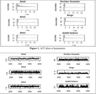
Hypothesis testing regarding the regression coefficients and mean responses are also straightforward. The program codes are available from the authors upon request. When the MCMC implementation is applied to the simulated data (see the Simulation Study section), the convergence of the MCMC samples is assessed using standard tools within WinBUGS such as trace plots and autocorrelation function (ACF) plots, as well as the Gelman-Rubin [17] convergence diagnostic.

Simulation Study

In this section, we study through some intensive simulation experiments, the behavior of the Bayesian estimators based on the square root of MSE and relative bias. We performed the simulation of the spatial beta regression model by assuming a GRF whose covariance structure is given by (6) while incorporating different scenarios for the spatial parameter. Consider the model

| , , ~ ( , (1 − ) ), = 1, … , ,

| , ~ (0, Σ ),

where β = (β , β , β ) and log = = x β +

τ = η. The values of the covariates and were

generated from a uniform distribution on the unit interval referring to [8], and we set, β = (−1,

2, −1.5) and ϕ=50. On the other hand, we consider the

spatial variance = 0.5 and different spatial range settings; ψ =0.1, 0.45 and 0.9. These values are considered after an initial study of the spatial parameters and we find out that the natural prior for the range parameter overestimates the aimed parameter in the case of spatial beta regression, so we attempt to estimate small values of the range.

Additionally, we consider different settings for the precision parameter , generating two possible models. Box-1

2 2 2

1 1

( , , ,

, ,

)

n

(

i i

, , )

n

(

i

, ,

, )

( ) ( ) (

) ( ) ( ).

i i

f

β δ

α σ λ

τ

f y

τ

β δ

f

τ

β

α σ λ

f

β

f

α σ λ

f

f

λ δ

f

= =

∝

∏

∏

×

y

Vol. 29 No.

Model 1: Model 2: l

In order to study was parameters o that would each scenario

Set 1.

ϕ~Gamma(

we have σ |

to find a prio aimed value therefore α =

Set 2.

ϕ~Gamma( σ ~Gamma

To illustra estimators, w regularly spa 10]×[0, 10] a

First, we parameter (M

2 Spring 201

=ϕ,

log(ϕ ) = δ

o evaluate our conducted fo of prior distrib

provide noni o are defined

β ~N(0,100

0.01,0.01) w

λ~exp(λ), λ~

or for small va for ψ lyin

= −Ln(ψ)~U β ~N(0,100

0.01,0.01) w

a(0,0.01) and

ate the effect we consider di aced grid, whi and [0, 15] ×

study the m Model 1). For

18 L.

+ δ z

r proposal pri or two sets butions were sp

informative p as follow.

0) for

whereas for s

~N(0, σ )I(0,

alues of the ran ng in the (0.

U(−4.5, 2.3).

0) for

with spatial par

d ψ ~U(0.01

t of sample s ifferent locati ich consist of

[0, 15]. model with a

the generated

Fi

Kalhori Nadra

iors, a simulat of priors, pecified in a w priors. Priors

r j=0, spatial parame

∞). We attem nge and have 01, 10) interv

r j=0,

rameter given

1, 10). size on Bayes

ons defined o f [0,5]× [0,5], fixed precis d data set of s

Figure 1.

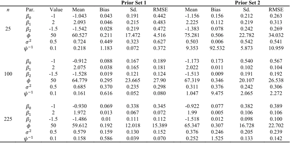
igure 2. Trace p

abadi and M. M

tion and way for 1,2, meter mpt our rval, 1,2, n by sian on a , [0, sion size 22 par elim avo siz 500 cha the sm and To pro ran Th 1.2 sta of dia Plo bet Ma

. ACF plots of p

plots of the esti

Mohhamadzad

5, we simula rameter, disre minate the e oid correlatio ze 100. Thus w

0, and the po ains are mixe e model, , so maller sample s Diagnostic te d there was n o validate this oportional red ndom initial v he resulted MP

2, indicating th atistics [26] al

Gibbs sampl agnostics wer ots of autocor tween distinct Figure 2 disp arkov chain

parameters

imated paramet

deh.

ate one chain egarding the ffect of the on problems w

we obtained a osterior infere ed slowly espe o we need to c

sizes to reach ests of conve no evidence of assertion, we duction factor. values were PRF is equal t

hat the chains lso show the lers for each re done using rrelation in Fig

t replication fo lays another t convergence

ers

J.

of size 100, first 50,000 initial values we considere an effective s ence is based ecially for th consider more convergence. ergence were f divergence have used th . Two chains generated sim to 1.02 which s are converge

convergence parameter. T g the Coda p

gure 1 show or estimating p tool employed

on all param

Sci. I. R. Iran

,000 for each iterations to s. Further, to ed spacing of ample of size on this. The e intercept of e iterations for implemented of the chains. e multivariate with different multaneously. is lower than ent. Geweke's of the results The reference package in R. independence parameters. d to assess the meters. Trace

plots showed that the chains have a stable performance around the true parameter value.

We computed the relative bias (RelBias) and the square root of MSE (RMSE) for each parameter over the 50 simulated samples. They are defined as

RelBias( ) = ∑ − 1 and RMSE( ) =

∑ −

Where θ = (β , β , β , ϕ, σ , ψ )and θ is the posterior estimate of θ for the ith sample. Table [1] presents the summary results for the estimation of all the parameters. It seems that the spatial variance is overestimated or underestimated according to the first and second sets of priors respectively. Nevertheless, it is worth mentioning that using a hierarchical prior for spatial variance, resulted in a reduction in the RelBias

and RMSE values when the sample size is increased. Moreover, bounded uniform distribution on the logarithm of the range resulted in proper estimates. This prior has solved the problem of over estimation and has also reduced the RelBias and RMSE in comparison with uniform prior density, especially for small sample sizes.

Another important aspect that should be assessed is the performance of the Bayesian estimators for other values of the spatial range when the sample size is small. The data generation scheme is similar to the simulation study described above, whereas other values for the range parameter are considered. Table 2 summarizes the numerical results of our simulation study over a 5×5 lattice, where the RelBias and the RMSE of the parameter estimators of Set 1 are smaller than Set 2. Hence we can conclude that our method

Table 1. Estimates of the parameters of Model 1 for different priors and sample sizes

Prior Set 1 Prior Set 2

n Par. Value Mean Bias Sd. RMSE Mean Bias Sd. RMSE -1 -1.043 0.043 0.191 0.442 -1.156 0.156 0.212 0.263 2 2.093 0.046 0.215 0.483 2.225 0.112 0.219 0.313 25 -1.5 -1.542 0.028 0.219 0.472 -1.383 0.078 0.242 0.269 50 60.527 0.211 17.472 4.516 75.281 0.506 22.782 34.032 0.5 0.724 0.449 0.323 0.627 0.503 0.006 0.542 0.541 0.1 0.218 1.183 0.072 0.372 9.353 92.532 5.873 10.959 -1 -0.912 0.088 0.167 0.189 -1.173 0.173 0.540 0.567 2 2.075 0.038 0.165 0.181 2.022 0.011 0.102 0.104 100 -1.5 -1.528 0.019 0.121 0.124 -1.513 0.009 0.191 0.192 50 64.779 0.295 23.665 27.90 67.319 0.346 20.107 26.538 0.5 0.685 0.370 0.235 0.298 0.311 0.376 0.242 0.306 0.1 0.161 0.616 0.052 0.080 1.047 9.475 2.065 2.272 -1 -0.930 0.069 0.338 0.345 -0.922 0.077 0.382 0.389 2 1.972 0.013 0.067 0.072 1.99 0.005 0.106 0.106 225 -1.5 -1.486 0.01 0.111 0.112 -1.518 0.012 0.098 0.100 50 59.612 0.192 12.018 15.389 65.347 0.307 16.728 22.702 0.5 0.579 0.159 0.130 0.152 0.376 0.246 0.205 0.239 0.1 0.158 0.586 0.039 0.070 0.252 1.525 0.133 0.142

Table 2. Estimates of the parameters of Model 1 for different priors and different values of spatial range

Prior Set 1 Prior Set 2

Par. Value Mean Bias Sd. RMSE Mean Bias Sd. RMSE -1 -0.903 0.097 0.223 0.243 -1.696 0.131 0.166 0.257

2 1.939 0.030 0.266 0.273 2.792 0.396 0.262 0.835 -1.5 -1.568 0.045 0.218 0.228 -0.901 0.399 0.215 0.636 50 33.233 0.335 9.899 19.470 44.288 0.114 11.558 12.893 0.5 0.637 0.273 0.263 0.296 0.123 0.754 0.059 0.382 0.45 0.361 0.199 0.166 0.188 14.046 30.213 3.914 14.148

Vol. 29 No. 2 Spring 2018 L. Kalhori Nadrabadi and M. Mohhamadzadeh. J. Sci. I. R. Iran

exhibits good performances in the estimation of the range parameter.

To explore how Bayesian estimates are affected by less informative priors, a sensitivity analysis was conducted. So applying vague priors, we use the following elicitation of prior distributions

β ~N(0,1000) for j=0,1,2, ϕ~Gamma(0.001,0.001)

and λ~N(0, 1000)I(0, ∞).

The results of this assessment are given in Table [3]. It can be observed that estimation of the parameters is not significantly affected by the use of less informative priors. In conclusion, the sensitivity analysis, convergence tests, plots and results over the 50 simulated data sets indicate that our results are reliable and can be applied to analyze real data sets when the basic circumstances of the model are met.

After investigating Model 1, we expended considerable effort to develop an SBGLMM model, assuming that the precision parameter is not fixed and then going on to examine different scenarios for parameter estimation. Consider the spatial beta regression model presented in (5) and suppose that

log(ϕ ) = z δ. As mentioned before, in Model 2 we

have log(ϕ ) = δ + δ z . Table 4 shows the outcomes

of our simulation study for Model 2 assuming

δ ~N(0,100) for j = 0, 1 and a prior distribution for

other parameters are the same as when assuming the precision parameter is fixed. In this state, we consider two samples in the regular grid, namely, 10 ×10 and 15× 15, then RelBias and RMSE of each parameter are computed over the 50 simulated samples.

From Table 4, we find out that δ and δ are not estimated properly for the sample of size 100. In order to obtain better estimates for these parameters, we examine different priors such as non-informative uniform prior distribution for each δ, and a zero mean t-student distribution with large variance and 3 degrees of freedom [27], i.e., we assume that δ ~t(0,100,3). Our motivation to use these priors was implementing a flat prior and a prior with heavier tails in comparison with normal distribution in order to treat extreme values if they exist. These suggested priors were not achieving proper estimates, so for the sake of brevity, outcomes are not presented here.

[8] utilized an exponential prior for degrees of freedom in t-student distribution, while setting a hierarchical prior for the random effect in the mixed beta regression model. Borrowing this idea for fixed effects, we assume a hierarchical prior for regression coefficients, that is δ ~t 0,100, ς where ς ~exp(0.1). Considering these priors the joint posterior distribution is given by (Box-2).

Table 3. Summary results of sensitive analysis for estimation of the parameters of Model 1

n = 100 n = 225

Par. Value Mean Bias Sd. RMSE Mean Bias Sd. RMSE -1 -0.830 0.170 0.337 0.377 -1.042 0.042 0.152 0.158 2 2.067 0.033 0.161 0.175 2.040 0.020 0.125 0.132 -1.5 -1.551 0.034 0.130 0.140 -1.509 0.006 0.123 0.123 50 90.146 0.803 39.974 56.654 80.184 0.604 39.184 49.462 0.5 0.679 0.357 0.218 0.282 0.411 0.178 0.187 0.207 0.1 0.364 2.643 0.213 0.340 0.192 0.923 0.087 0.127

Table 4. Estimates of the parameters of Model 2 for different priors and sample sizes

Prior Set 1 Prior Set 2

Posterior i sampling m distributions. work proper simulation re Values of po that the su appropriately

From Tab Normal, t-s distributions the correspo addition, Re Therefore, i distributions estimation of Normal distr suitable prior parameter m of the sensi priors can b involved in implied to an an applicatio Application o

As an ap available fro Survey (HIE provide infor aims to prov expenditure f and national households distributiona HIES has b

Box-2

Par.

inference is m method on . Since these l rly for the sa esults for n = 2 osterior mean uggested prio

y.

ble 4 and 5, it student and

for δ, the ob onding true v elBias and R

it can be do not mak f δ. According ribution for th

r for regressio model requires itivity analysi be used for

an SBGLM nalyze a real on of our prop on HIES data pplication, w om the Househ ES) of Iran, wh rmation about vide estimate for urban and

levels. Makin income, exp l patterns, th een applied t

Value -1 2 -1.5 4 -0.4 0.5 0.1

made up by ap related f latest prior dis ample of size 225 are presen , RelBias and ors are able t can be seen hierarchical btained estim values of th RMSE are re concluded th ke significan gly, it is sugge e sake of simp on coefficients s further resea is indicate th estimation of MM. Hence, t data set prov osed model. a

we consider hold Income hich is an imp t national acc s of the aver rural househo ng it possible t

penditure co he informatio to calculate p

Table 5. Sum

Mean B -0.921 -0

2.105 0 -1.540 0 4.148 0 -0.369 -0 0.204 -0 0.434 3

pplying the Gi full conditio stributions do es 100, only nted in Table d RMSE indic

to estimate that by apply t-student p ates are close he parameter. elatively simi hat these p nt differences ested to apply plicity. Findin s of the precis arch. The res hat the propo f the parame these priors ided by HIES

the informat and Expendit portant survey ounts. The HI rage income olds at provin to learn about omposition,

on provided poverty line mmary results o

t- stu

Bias Sd. 0.079 0.08 .052 0.08 .027 0.07 .037 0.44 0.076 0.73 0.592 0.10 .336 0.21

ibbs onal not the [5]. cate e δ

ying prior e to In ilar. prior s in y the ng a sion sults osed eters are S as tion ture y to IES and ncial t the and by and stu Th its rot all and sam sur to yea the Th Te ava acc req exp hou Th situ res a cov De of Nu (N dep the res cov the mo cov We of modelling bot

udent

. RMSE 89 0.119 83 0.133 79 0.089 41 0.465 30 0.731 01 0.313 19 0.399

udy the impur he HIES has a survey whic tating panel d

private and d rural areas mpling unit re rveys and then obtain more ar, the sample e year, so eac he working da hran provided ailable due to cess from the quest. The re

penses spent use-hold duri his proportion uation of hou sponse variabl

better econo variates prov ecile of Incom Housing Uni umber of Em

EM). The M pendency, so e data. Figur sponse variabl In order to variates on th e backward el odel and at

variate until a e initially su th parameters o E Me -0. 1.9 -1. 4.2 -0.2 0.6 0.1

rity in househ three-stage cl ch is conduc design and its collective se . In a 0-5 ro emains in the n goes out of t representativ es are distribu ch month som

ta set is a sele d by HIES. T o the privacy e correspondin

esponse varia on food to t ing the refer can be used useholds. We le gets lower v omic status. vided by HIE me (DI) , the H it (AHU), Ho mployed Mem Moran-I test s

we adopted re [3] shows le in Tehran.

extract the he response v limination pro each step r all remaining uggest using

of Beta density

Hi

ean Bia 846 -0.1 996 -0.0 501 0.00 209 0.05 235 -0.4 664 0.32 111 0.1

hold income a luster samplin cted annually target popula ettled househo otating panel

sample for fi the survey for ve estimates

uted across th me samples ar

ected subset o The dataset is policy of SC ng author on able is the p the total exp rence month d for explorin e expect that

values for hou The poten ES questionn Household Siz ousehold Inco mbers of th showed signi SBGLMM f s the spatial best subset variable, we p ocedure startin remove a no covariates ar the following

ierarchical t-st

as Sd. 154 0.394 002 0.100 01 0.132 52 1.103 413 1.325 28 0.271 15 0.065

and facilities. ng method for y with a 0-5 ation includes olds in urban design, each ive sequential rever. In order of the whole he months of re considered. of the data for s not publicly CI but it is in a reasonable proportion of enditure of a of sampling. g the welfare t our desired useholds with ntially useful naire are the ze (HS), Area ome (HI) and he household ificant spatial for modelling map of the of effective proceed using ng by the full on-significant re significant. g full spatial

Vol. 29 No.

model (Box-The Varia check the regressors. T the assumed there is no s mentioned in analysis and the proposed sample size application, precision

ϕ~Gamma(

parameter, w

and α = −Ln

To estima the 800,000 size 100. Th which the po model is th procedure.

log

Box-3

Full Mode

Par.

2 Spring 201

3).

ance Inflation multicollinea The largest VI d covariates a

ignificant evi n results of th

convergence d priors to

s. So we u i.e., β~N (0

parameter

0.01, 0.01). we have σ |λ

n(ψ)~U(−4.5

ate the parame values of the hus, we have a osterior inferen he outcome o

1 − =

el : log(

1

i

μ

μ

−

18 L.

n Factor (VIF) arity problem

IF value is 3. are included i dence of mul he simulation tests indicate analyze SBL use the same

, 10 I ) and is In addition,

λ~exp(λ), λ~ 5, 2.3). eters, we burn e chain consid a total of 3,00 nce is based o of the backw

+ +

0 1

)

i

μ

β β

μ

= +

Figure

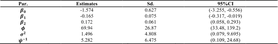
Table 6. P

Estimat -1.574 -0.165 0.172 69.94 1.496 5.282 Kalhori Nadra

) is calculated m between

.33(<5) when in the model, ticollinearity. n study, sensit

e that we can LGMM in sm

e priors in assume that

fixed w for the spa

~N(0, σ )I(0, ∞

ned-in 500,000 dering spacing 00 samples up on. The follow ward eliminat

+

2

i i

DI

HS

β

+

β

e 3. Spatial plot Parameter estim tes 4 5 2 4 6 2

abadi and M. M

d to the n all , so As tive use mall the the with atial ∞), 0 of g of pon wing tion cor ran eva DI 13 the the cre an cov sig inc the dec me sm com

3

AHU

i

β

+

+

t of response va mates, Sd. and 9

Sd. 0.62 0.07 0.06 26.8 4.80 6.47 Mohhamadzad

To evaluate rrelation struc ndom effect fr

log 1

The deviance aluating the p

C criteria for 8.007, respect e model contai e data.

Table [6] sh edible inte

d ψ parame

variates hous gnificant. Inc

creasing the p e total expend cile of incom eans that hou maller propor mparison with

4

HI

i 5

N

β

+

β

+

ariable in Tehra 95% CI for Mod

. 27 75 61 87 08 75 deh.

the effective cture in the s rom the model

1 − = +

e information performance r models (7) tively. So acc ining the spati hows the post erval (CI) eters. It can sehold size a creasing hou proportion of diture of a hou me the propo useholds with tion of thei h households

,i

i i

NEM

+

τ

an city del Step 4

(-3 (-0 (0 (3 (0 (0 J.

eness of incl study, we om l in (7) and fit

+ +

criterion (DIC of the fitted and (8) are -cording to the ial random eff terior mean a for th n be seen t and decile of

usehold size expenses spe usehold. By i ortion will be h more incom ir expenses s with a weak

1, , 57

= …

95%CI .255, -0.556) 0.317, -0.019) 0.058, 0.293) 3.48, 139.2) 0.079, 9.695) 0.109, 24.68)

Sci. I. R. Iran

uding spatial mit the spatial

t it again.

C) is used for models. The 160.52 and -e DIC crit-eria, ffect better fits and the 95%

e β, ϕ, σ ,

that the two f income are e results in nt on food to increasing the e reduced. It me allocate a to food in ker economic

status.

It is important to note that adding spatial effect is necessary to study the response variable. Because ignoring the spatial correlation results in increasing the DIC value, it means that if the spatial dependency of the response variable is neglected, the model is not well fitted.

Results and Discussion

In cases of working with spatially correlated data, this property should be considered in the data analysis to prevent arriving at misleading results. Our proposed SBGLMM is applicable when the spatial response variable is beta distributed. The reparametrized beta distribution has two parameters namely, the mean and the precision parameter. We consider SBGLMM in two situations. First, we assumed that the precision parameter is fixed and then the model was extended for a varying precision parameter status. The spatial correlation structure was included in the model using a random effect in the mean model. After doing an initial study and realizing that typical priors in the Bayesian context are unable to estimate small values of the spatial range parameter, we made an effort to find a suitable prior for this parameter. To analyze the sensitivity of priors, an intensive simulation study carried out upon which the proper values of hyper parameters were assigned. The Bayesian approach was applied to estimate the parameters involved in the proposed model. As the posterior distribution is complicated, the Gibbs sampler was run to fit the model using MCMC scheme, while facing slow mixing chains. The further inference was performed considering convergence tests and graphical diagnostic tools. Outcomes of intensive simulation studies over different sample sizes and results of sensitivity analysis, demonstrated that parameter estimations are reliable based on the proposed priors which are working properly, especially for small values of spatial range even for small sample sizes.

Additionally, we targeted to fit a model while a varying precision parameter is supposed. The linear pattern including fixed effects is assumed for the precision parameter. Finding proper priors for these regression coefficients was challenging and time consuming. Although Normal prior distribution does not provide appropriate estimates for the regression coefficients when the sample size is small, results of simulations confirm that Normal prior distribution is able to estimate regression parameters of the precision model when the sample size is increased.

SBGLMM provides us with a useful tool for

modelling spatially correlated rates and proportions which are common in many areas such as official statistics. As an application, we used our model to study HIES data in Tehran, the capital of Iran. The results show that the proportion of expenses spent on food in a household is affected by decile of income and household size. It is worth to mention that due to the spatial dependency of the response variable, adding the spatial effect to the model yielded to get better results.

There is a wide vicinity for future work on this issue. For instance, this can be carried out by extending the models including some other random effects, working on other spatial correlation structures, or studying spatiotemporal issues.

Acknowledgement

The authors are thankful to the referees for their many helpful comments that greatly improved this paper . We also wish to acknowledge for the support from Center of Excellence of Spatio-Temporal Data Analysis in Tarbiat Modares University .

References

1. Ferrari S., Cribari-Neto F. Beta Regression for Modelling Rates and Proportions. J. Appl. Stat. 31: 799-815 (2004). 2. Ferrari S.L., Pinheiro E.C. Improved Likelihood Inference

in Beta Regression. J. Stat. Comput. Simul. 81: 431-443 (2011).

3. Cepeda-Cuervo E., Gamerman D. Bayesian Methodology for Modelling Parameters in the two Parameter Exponential Family. Rev. Estad. 57: 93-105 (2005).

4. Smithson M., Verkuilen J. A Better Lemon Squeezer? Maximum-Likelihood Regression with Beta Distributed Dependent Variables. Psychol. Methods. 11: 54-71 (2006). 5. Branscum A.J., Johnson W.O., Thurmond M.C. Bayesian

Beta Regression: Applications to Household Expenditure Data and Genetic Distance Between Foot-and-Mouth Disease Viruses. Aust. N. Z. J. Stat.49: 287-301 (2007). 6. Simas A.B., Barreto-Souza W., Rocha A.V. Improved

Estimators for a General Class of Beta Regression Models.

Comput. Stat. Data Anal. 54: 348-366 (2010).

7. Zimprich D. Modelling Change in Skewed Variables using Mixed Beta Regression Models. Res Hum Dev. 7: 9-26 (2010).

8. Figueroa-Zúñiga J.I., Arellano-Valle R.B., Ferrari S.L. Mixed Beta Regression: A Bayesian Perspective. Comput. Stat. Data Anal. 61: 137-147 (2013).

9. Verkuilen J., Smithson M. Mixed and Mixture Regression Models for Continuous Bounded Responses using the Beta Distribution. J. Educ. Behav. Stat.37: 82-113 (2012). 10.Ferreira G., Figueroa-Zúñiga J.I., de Castro M. Partially

Linear Beta regression Model with Autoregressive Errors.

TEST. 24: 752-775 (2015).

Vol. 29 No. 2 Spring 2018 L. Kalhori Nadrabadi and M. Mohhamadzadeh. J. Sci. I. R. Iran

Generalized Spatial Econometric Models. Commun. Stat. Simul. Comput.41: 671-685 (2012).

12.Cepeda-Cuervo, E., Nunez-Anton V. Spatial Double Generalized Beta Regression Models Extensions and Application to Study Quality of Education in Colombia. J. Educ. Behav. Stat.38:604-628 (2013).

13.Gholizadeh K., Mohammadzadeh M., Ghayyomi Z. Spatial Analysis of Structured Additive Regression and Modelling of Crime Data in Tehran City Using Integrated Nested Laplace Approximation. Journal of Statistical Society. 7: 103-124 (2013).

14.Fustos R. Modelo Lineal Generalizado Espacial Con Variable Respuesta Beta. Engineer's Degree Dissertation. Department of Statistics. University of Concepcion, Chile. (2013).

15.Lagos-Alvarez B.M., Fustos-Toribio R., Figueroa-Zúñiga J., and Mateu, J. Geostatistical Mixed Beta Regression: A Bayesian Approach. SERRA. 31: 571-584 (2016).

16.Kalhori L., Mohammadzadeh M. Spatial Beta Regression Model with Random Effect. J. SRI. 13: 214-230 (2016). 17.Brooks S.P., Gelman A. General Methods for Monitoring

Convergence of Iterative Simulations. J. Comput. Graph. Stat.7: 434-455 (1998).

18.Heidelberger P., Welch P.D. A Spectral Method for Confidence Interval Generation and Run Length Control in Simulations. Commun. ACM. 24: 233-245 (1981).

19.Diggle P.J., Tawn J., Moyeed R. Model-Based

Geostatistics. J. Royal. Stat. Soc: Ser. C Appl. Stat. 47: 299-350 (1998).

20.Mark S. Handcock M.L.S. A Bayesian Analysis of Kriging.

Technometrics. 35: 403-410 (1993).

21.Stein M.L. Interpolation of Spatial Data: Some Theory for Kriging, Springer Science & Business Media, New York.

(2012).

22.Stein M.L. Interpolation of Spatial Data: Some Theory for Kriging, Springer Science & Business Media, New York.

(2012).

23.Chen M.H., Shao Q.M., Ibrahim J. Monte Carlo Methods in Bayesian Computation, Springer, New York. (2000). 24.Sturtz S., Ligges U., Gelman A. R2winbugs: A Package

for Running Winbugs from R. J. Stat. Softw. 12: 1-16 (2005).

25.R Core Team. R: A Language and Environment for Statistical Computing. R Foundation for Statistical Computing, Austria, Vienna. (2013).

26.Geweke J. Evaluating the Accuracy of Sampling Based Approaches to the Calculation of Posterior Moments. Federal Reserve Bank of Minneapolis, Research Department Minneapolis, MN, USA. 196: (1991).

27.Huang X., Li G., Elashoff R.M. A Joint Model of Longitudinal and Competing Risks Survival Data with Heterogeneous Random Effects and Outlying Longitudinal Measurements. Stat. Its Interface. 3: 185 (2010).

Appendix I:

Full conditional distributions are as follow

2 0

1

(

,

, , , , )

y

(

, , )

y

(

,

,

)

( )

n

i i i

f y

π

β

α σ λ φ

τ

π

β τ

φ

τ

β

φ π β

=

∝

∝

∏

∣

∣

∣

1

0 0 0

1

(

) '

(

)

exp(

log( (

, , ))

)

2

n

i i i

f y

τ

β

φ

β

β

−

β

β

=

−

Σ

−

=



∣

−

2 2

0 0

(

, , , , , )

y

(

, , )

π σ

∣

β

α λ φ

τ

∝

π σ

∣

α

λ

τ

∝

π

(

τ

∣

α λ σ π σ λ π λ

, ,

₀2

) (

₀2

∣

) ( )

exp

1

(

1

) exp(

₀2

) exp

1

)

2

2

'

2

(

λ τ

λ

λ μ

λ

λσ

σ

τ

−

τ

−

−

−

=

Σ

−

2 2 2

0 0 0

(

,

, )

(

, ,

) (

) ( )

π α λ σ τ

∣

∝

π τ α λ σ π σ λ π α

∣

∣

1

2 1

1

2 1

1

exp

(

)

2

1

exp

(

2 ln(

))

2

'

'

τ

τ

τ

τ

τ

τ

−

−

Σ

Σ

−

=

−

−

=

+

−









2 0

2 0

1 2

2

0 ( , , )

( , , ) ( ) 1

exp {( ' ) ( )

2

( , , , , ,y)

λ τ

λ π λ σ α

π α λ σ π λ

λ μ σ τ

τ

τ τ

π λ β σ α φ

τ

−

∝ ∝

− −

= Σ +

∣ ∣

∣

2

0

y

(

β

,

, , , , )

τ

(

β

, , )

y

π φ

∣

σ α λ

∝

π φ

∣

τ

1 1

1

1

2 2

1 1

(

, , ) ( )

1

exp(

log( (

, , )

)

.

n

i i i

n

i i i

f y

f y

β

β

τ

φ π φ

τ

φ φ

φ

=

−

=

∝

=

−

∏



∣

∣

ò

ò

ò ò

ò

2 2

0 0

2 0 1

(

, , ,

, , , )

(

, ,

, , )

(

, , ) (

, ,

, )

k k k k

n

i i k k i

y

y

f y

π τ τ β α σ λ φ

π τ τ α σ λ

τ β φ π τ τ α σ λ

− −

− =

∝

∝

∏

∣

∣

∣

∣

1

≤ ≤

k n