Semantic and generic object segmentation for scene analysis using RGB-D Data

(1)

Semantic and generic object segmentation

for scene analysis using RGB-D data

by Xiao Lin

ADVERTIMENT La consulta d’aquesta tesi queda condicionada a l’acceptació de les següents condicions d'ús: La difusió d’aquesta tesi per mitjà del r e p o s i t o r i i n s t i t u c i o n a l UPCommons (http://upcommons.upc.edu/tesis) i el repositori cooperatiu TDX (h t t p : / / w w w . t d x . c a t /) ha estat autoritzada pels titulars dels drets de propietat intel·lectual

únicament per a usos privats emmarcats en activitats d’investigació i docència. No s’autoritza

la seva reproducció amb finalitats de lucre ni la seva difusió i posada a disposició des d’un lloc aliè al servei UPCommons o TDX. No s’autoritza la presentació del seu contingut en una finestra o marc aliè a UPCommons (framing). Aquesta reserva de drets afecta tant al resum de presentació de la tesi com als seus continguts. En la utilització o cita de parts de la tesi és obligat indicar el nom de la persona autora.

ADVERTENCIA La consulta de esta tesis queda condicionada a la aceptación de las siguientes condiciones de uso: La difusión de esta tesis por medio del repositorio institucional UPCommons (http://upcommons.upc.edu/tesis) y el repositorio cooperativo TDR ( http://www.tdx.cat/?locale-attribute=es) ha sido autorizada por los titulares de los derechos de propiedad intelectual

únicamente para usos privados enmarcados en actividades de investigación y docencia. No se autoriza su reproducción con finalidades de lucro ni su difusión y puesta a disposición desde un sitio ajeno al servicio UPCommons No se autoriza la presentación de su contenido en una ventana o marco ajeno a UPCommons (framing). Esta reserva de derechos afecta tanto al resumen de presentación de la tesis como a sus contenidos. En la utilización o cita de partes de la tesis es obligado indicar el nombre de la persona autora.

WARNING On having consulted this thesis you’re accepting the following use conditions: Spreading this thesis by the i n s t i t u t i o n a l r e p o s i t o r y UPCommons (http://upcommons.upc.edu/tesis) and the cooperative repository TDX ( http://www.tdx.cat/?locale-attribute=en) has been authorized by the titular of the intellectual property rights only for private uses placed in investigation and teaching activities. Reproduction with lucrative aims is not authorized neither its spreading nor availability from a site foreign to the UPCommons service. Introducing its content in a window or frame foreign to the UPCommons service is not authorized (framing). These rights affect to the presentation summary of the thesis as well as to its contents. In the using or citation of parts of the thesis it’s obliged to indicate the name of the author.

(2)

Universitat Polit`

ecnica de Catalunya

Departamento de Teoria del Senyal i Comunicacions

Semantic and Generic Object Segmentation for

Scene Analysis Using RGB-D Data

by

_{Xiao Lin}

Doctoral Thesis

Advisors: Josep Ramon Casas and Montse Pard`

as

(3)

(4)

Abstract

In this thesis, we study RGB-D based segmentation problems from different per-spectives in terms of the input data. Apart from the basic photometric and geometric information contained in the RGB-D data, also semantic and temporal information are usually considered in an RGB-D based segmentation system.

The first part of this thesis focuses on an RGB-D based semantic segmentation problem, where the predefined semantics and annotated training data are available. First, we review how RGB-D data has been exploited in the state-of-the-art to help training classifiers in semantic segmentation task. Inspired by these works, we follow a multi-task learning schema, where semantic segmentation and depth estimation are jointly tackled in a Convolutional Neural Network (CNN). Since semantic segmenta-tion and depth estimasegmenta-tion are two highly correlated tasks, approaching them jointly can be mutually beneficial. In this case, depth information along with the segmenta-tion annotasegmenta-tion in the training data helps better defining the target of the training process of the classifier, instead of feeding the system blindly with an extra input channel. We design a novel hybrid CNN architecture by investigating the common attributes as well as the distinction for depth estimation and semantic segmentation. The proposed architecture is tested and compared with state-of-the-art approaches in different datasets.

Although outstanding results are achieved in semantic segmentation, the limita-tions in these approaches are also obvious. Semantic segmentation strongly relies on predefined semantics and a large amount of annotated data, which may not be avail-able in more general applications. On the other hand, classical image segmentation tackles the segmentation task in a more general way. But classical approaches hardly obtain object level segmentation due to the lack of higher level knowledge. Thus, in the second part of this thesis, we focus on an RGB-D based generic instance segmenta-tion problem where temporal informasegmenta-tion is available from the RGB-D video while no semantic information is provided. We present a novel generic segmentation approach for 3D point cloud video (stream data) thoroughly exploiting the explicit geometry

(5)

and temporal correspondences in RGB-D. The proposed approach is validated and compared with state-of-the-art generic segmentation approaches in different datasets. Finally, in the third part of this thesis, we present a method which combines the advantages in both semantic segmentation and generic segmentation, where we discover object instances using the generic approach and model them by learning from the few discovered examples by applying the approach of semantic segmentation. To do so, we employ the one shot learning technique, which performs knowledge transfer from a generally trained model to a specific instance model. The learned instance models generate robust features in distinguishing different instances, which is fed to the generic segmentation approach to perform improved segmentation. The approach is validated with experiments conducted on a carefully selected dataset.

(6)

Acknowledgments

I would like to acknowledge the help, support and guidance of my thesis advisors, Professor Josep Ramon Casas and Professor Montse Pard`as, with the most sincere gratitude. They offered me the freedom to work on the research subject I like and explore it, always encouraged me to keep trying when I wanted to give up. I could not have imagined having a better advisors and mentors.

I am very grateful to my groupmates in the Image Processing Group (GPI) of Signal Theory and Communications Department (TSC) of UPC for the help and support in all the time of research. I also want to acknowledge the technical support from Albert Gil Moreno and Josep Pujal.

I am indebted to my parents and my loving wife, Yi Sun, for their always uncondi-tional support and encouragement. Their love has provided me with the enthusiasm to rise to the challenges and conquer them.

Finally, I want to thank the finance support from the Joint China Scholarship Council (CSC)-Universitat Polit`ecnica de Catalunya (UPC) Scholarship and the projects BIGGRAPH (TEC2013-43935-R) and MALEGRA (TEC2016-75976-R).

(7)

List of Figures

1.1 An example of the manual segmentation result of a color image . . . . 3

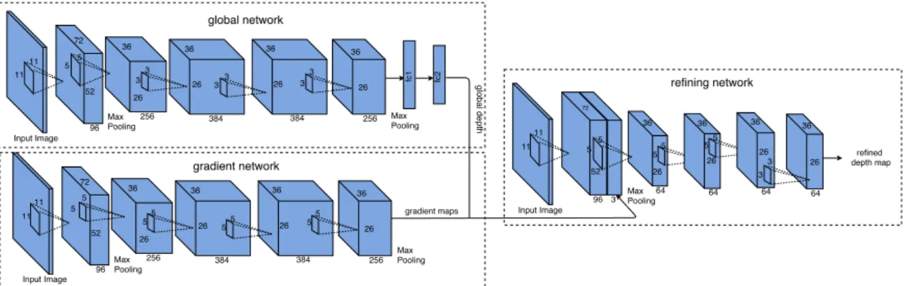
3.1 Depth estimation network. . . 36

3.2 Semantic segmentation network. . . 37

3.3 Architecture 1 . . . 38

3.4 Architecture 2 . . . 39

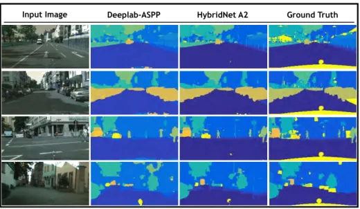
3.5 Semantic segmentation qualitative results. A comparison between se-mantic segmentation estimation against ground truth is presented. From left to right, input image is depicted in the first column. In column 2 the segmentation map estimated by DeepLab-ASPP semantic tation network [SZ14] is presented, in column 3 the estimated segmen-tation map by our hybrid method are presented and finally the ground truth is depicted in column 4. . . 46

3.6 Depth estimation qualitative results. A visual comparison between the estimated depth maps against the ground truth is presented. In the first column is presented the input image, columns 2 and 3 depict the estimated depth maps obtained by DepthNet in [Iva16] and our hybrid model A2 respectively. Finally, ground truth is presented in column 4. . 49

3.7 A 2D example of failures in depth estimation metrics . . . 49

3.8 Semantic segmentation qualitative results. A comparison between se-mantic segmentation estimations against ground truth is presented. Input image is depicted in the first row. In the 2nd and 3rd are pre-sented the estimated segmentation mask obtained from HybirNet A2 and the ground truth respectively. . . 52

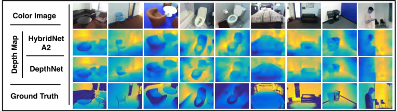
3.9 Depth estimation qualitative results. A comparison between depth estimations against ground truth is presented. Input image is depicted in the first row. In the 2nd and 3rd are presented the estimated depth map of our method and the ground truth respectively. . . 54

(11)

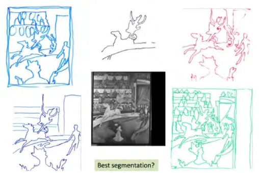
4.1 First row: input point clouds and color images. Second row: segmen-tation errors (false split in purple on left, false merge in red on the right) in challenging scenes with occlusions/self-occlusions or object interactions, and the corresponding sketch maps shown besides. Third row: Our segmentation result by analyzing generic features in spatio-temporal domain to handle the challenges without introducing neither strong prior knowledge nor initialization, together with the correspond-ing sketch maps. . . 61 4.2 An example of the super-voxels generated in our approach from a point

cloud with different seed density. (a) The color image, (b)Rseed = 0.06m, (c)Rseed = 0.1m, (d)Rseed = 0.15m. Each super-voxel is labeled with a random color. . . 65 4.3 An example of the super-voxels generated in our approach from a point

cloud. (a) The original point cloud. (b) The voxels (each super-voxel is labeled with a random color). . . 65 4.4 An example of plane detection results. The points in red, green and

blue belong to detected planes. The points in black are the points in the “not on any plane” class. (a) Plane detection result from [HHRB11]. (b) Plane detection result from our approach. . . 67 4.5 The hierarchical structure built for a point cloud. Different nodes at

the same level in the hierarchy are labeled with different colors. The point cloud beside it is labeled with the same color of its related node. 69 4.6 An overview of the proposed approach. . . 71 4.7 An example of hierarchical structure creation. Upper-left: Object

seg-mentation att−1 and its hierarchical structure; Middle column: color image at t, detected blobs in the point cloud at t, illustrations about the establishment of correspondences and blob segmentation process; Right: hierarchical structure building process att. . . 72 4.8 An example of temporal inconsistency problem. (a) The problem when

establishing the correspondences between components in the previous frame and blobs in the current frame. (b) Using the segments instead of components solves this problem. . . 74 4.9 Example of how we update the object segmentation in the current frame

by dynamically managing object splits (a) and merges (b) . . . 79 4.10 Qualitative results in RGB-D video foreground segmentation dataset . 84 4.11 An example of the segmentation result in our method: (a) a color image

(b) related segmentation mask . . . 85 4.12 Qualitative results of significant objects selection in RGB-D video

(12)

4.13 (a)-(b) present the IOU (vertical axis) per frame (horizontal) results for Seq 2-3. Red: our approach without DMMS, Blue: with DMMS.(c)-(d) present point cloud plots in frame 30 of Seq 2 and in frame 64 of Seq

3, object proposals are marked in different colors. . . 88

4.14 Qualitative results of the proposed method. Column 1-2: from human manipulation dataset in [PSPK14], Column 3: from data in [HDT15] and Column 4: from data recorded by ourselves. . . 89

4.15 Segmentation performance shown as mean IOU (vertical axis) over n frames (horizontal axis) in 4 different sequences. Red: method in [LCP16]. Blue: S-FC-CRF. . . 92

4.16 Segmentation performance verification: (a) on robustness to segmen-tation error for P-FC-CRF in green compared to CRF and S-FC-CRF in red and blue, (b) on employing different unary energy in S-FC-CRF, shown as mean IOU (vertical axis) over n frames (horizontal axis). Blue: S-FC-CRF with unary energy defined based only on difference in location. RED: S-FC-CRF with unary defined based on difference in color, local surface normal and location. . . 92

4.17 Quantitative results in error per frame for different sequences (a)-(d). Red point/line represents SV, blue point/line represents RNBLS . . . . 94

4.18 IoU scores for 20 validation images under different settings ofω1 . . . . 95

5.1 An example of blob segmentation in frametconsidering the temporally corresponded object instances in frame t−1. . . 101

5.2 The schema of proposed approach. . . 103

5.3 The architectures of the base network and extened network. . . 106

5.4 Examples of qualitative results from CNN+GIS in the first row and GIS in the second row. . . 109

A.1 The architecutre of AlexNet . . . 123

A.2 The architecture of VGGNet . . . 124

A.3 The architecture of a residual block . . . 124

B.1 An example of a factor graph . . . 126

(13)

(14)

Acronyms

ACM Active contour model. 25

AR Augmented Reality. 43

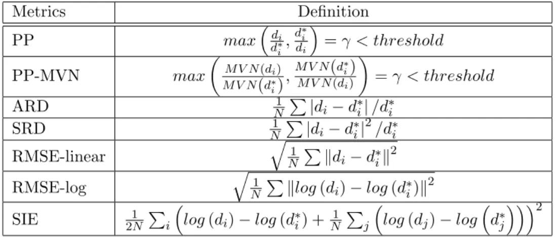
ARD Absolute Relative Difference. 48, 50, 54

ASMS Adaptive Surface Models based 3D Segmentation method. 86

ASPP Atrous Spatial Pyramid Pooling. 53, 106

BOV Bag of Visual Words. 17

BPT Binary Partition Tree. 30

C Class Average Accuracy. 47, 52, 56, 57

CNN Convolutional Neural Network. iii, 10–12, 16, 20–23, 28, 31, 33–35, 59, 97–99, 102, 103, 108, 110–112, 114–116, 119, 122, 123

CRF Conditional Random Field. 67, 68, 73, 77, 82, 90, 94, 114, 125–128

DeepLab-ASPP Deeplab-Atrous Spatial Pyramid Pooling. 37–39, 42, 45–47, 52–

54, 104, 106

DMMS Dynamic Management of Merge and Split. 82

FCN Fully Convolutional Network. 21, 23, 45, 53

FPFH Fast Point Feature Histograms. 18, 64

(15)

HOD Histogram of Oriented Depth. 18

ILSVRC ImageNet Large-Scale Visual Recognition Challenge. 122, 124

LRN Local Response Normalization layer. 40, 41

mIoU mean Intersection over Union. 47, 52, 57

PFH Point Feature Histogram. 18

PLEDL Pixel Level Enconding and Depth Layering. 23

PP Percentage of Pixel. 48, 54

PP-MVN Mean Variance Normalized Pixel of Percentage. 48, 54

ReLU Rectified Learnear Unit. 40, 41, 120, 121

RMSE-linear Linear Root Mean Square Error. 48, 54

RMSE-log Log Root Mean Square Error. 48, 54

RNG Random Number Generator. 42

SGD Stochastic Gradient Descent. 107, 122

SIE Scale Invariant Error. 48, 55

SIFT Scale Invariant Feature Transform. 17, 118

SLIC Simple Linear Iterative Clustering. 27

SRD Square Relative Difference. 48, 50, 54

SUN-RGBD RGB-D Scene Understanding Benchmark Dataset. 51

(16)

Chapter

1

Introduction and Overview

A visual scene is commonly defined as a view of an environment composed of ob-jects organized in a meaningful way, like a kitchen, a street or a forest path. More broadly, the domain of scene perception includes any visual stimulus that contains multiple elements arranged in a spatial layout, for example a shelf of books, an of-fice desk, or leaves on the ground. When a human vision system perceives a scene, several abilities are involved in the process, such as separating elements in the scene, identifying different elements or constructing spatial/temporal relationships between elements [Gol10].

In a computer vision system, a scene is information that flows from a physical environment into a perceptual system via sensory transduction [RB94, Gei08]. The usual information input for computer vision tasks is a color image. Color images capture a projection of the scene into the image plane with discrete values at each sampled pixel providing a dense color representation. The projective nature of imaging systems loses one dimension of the scene geometry. Therefore, adding the distance from a scene to the camera at each pixel brings back a highly informative feature. The distance information provides the 3D geometry, object poses and spatial layout of the projected scene. The distance information is usually encoded in a depth image, registered with a color image. A video formed as a sequence of color+depth images is also usually leveraged as a type of input. It provides the dynamics of a scene, that is to say, the temporal information of a scene is available for both photometry (color)

(17)

and geometry (depth). A color image and the registered depth image are paired as

an RGB-D frame. A video containing RGB-D frames is known as an RGB-D

video/stream. Mimicking the abilities of human perception in processing multiple

types of information, computer vision systems aim to endow machines with smart perception skills. In practice, several tasks in computer vision, such as segmentation, object detection and object recognition, usually deal with information fusion in some way.

In this thesis, we focus on solving segmentation problems with RGB-D data in a computer vision system. Segmentation is an essential task serving as the foundation for higher level problems such as object recognition and scene analysis. Regarding the involved information, we can categorize segmentation problems into several classes. In the following sections, a brief introduction for different segmentation problems are described, while the advantages and challenges of exploiting RGB-D data in such problems are discussed. In Section 1.1, we define static image segmentation tasks taking only photometric information as the input (RGB based) and those based on both photometric and geometric information (RGB-D based). In each case, we further categorize into unsupervised/supervised segmentation. Section 1.2 defines a video segmentation task and how RGB-D can help.

1.1 Static Image Segmentation

Image segmentation is an ill posed problem, since a unique solution does not exist. Fig.1.1 shows an example illustrating that different segmentation exists when performing manual segmentation of a color image. The criterion of a segmentation system varies regarding the final application.

1.1.1 RGB based Image Segmentation

In general, RGB based image segmentation is defined as a task in which the segmentation system F takes a color image I as input and outputs a segmentation

(18)

Figure 1.1: An example of the manual segmentation result of a color image

mask L, F (I) →L. The segmentation mask represents segments of the color image using different labels.

RGB based Unsupervised Image Segmentation

Image segmentation is traditionally defined as partitioning the image into a set of segments showing some sort of pixel homogeneity (known asunsupervised

segmen-tation or low level segmentation). The connected labels li of the segmentation

maskLcreate a partition{li}of the imageI, so that∪liis the complete image support and li∩lj = ø for alli 6=j. Usually, the labels optimize some segmentation criterion

C, so that C(li) =T rue for alli, andC(li∪lj) =f alsefor alli, j. Connectivity can be understood here as 4− or 8− connectivity over an square image grid.

In unsupervised segmentation approaches, pixels are usually grouped into segments according to the criterion C and regarding to their local homogeneity. The segments obtained in such low level segmentation approaches are more perceptually meaningful than raw pixels, while also producing a simplified representation of the image, which can be exploited by higher level segmentation and classification approaches. However,

(19)

obtaining high level segmentation such as object segmentation only based on unsu-pervised approaches is extremely difficult due to the lack of semantic information to define the segmentation criterion.

RGB based Supervised Image Segmentation

In order to produce more meaningful regions, whichideallycorrespond to semantic objects in the scene, high level supervision is usually incorporated into the process. Supervised image segmentation methods are based on image models or classifiers able to introduce semantic hints into the segmentation criterion. Semantics are introduced as a classification strategy defined through training from semantically enriched data elaborated or supervised by humans, such as predefined object models or annotated data. According to the supervision used in the methods, they are further catego-rized, such as model based segmentation, semantic segmentation, etc. Among them,

semantic segmentation is one of the hottest fields in the last decade. Semantic

segmentation aims to recognize the semantic category of the image at the pixel level. A classifier Θ is usually trained on a limited number of classes/semantics θ, in order to output the class label of each pixel L(x, y) (Θ (I, x, y |θ) → L(x, y)). x

and y denote the coordinates of the pixel in the image. The pixel classes resulting of a classification are, in principle, not necessarily connected, but a different label may be assigned to each connected component to get a segmentation partition that fulfills the definition above. However, training the classifier requires a large amount of annotated data, which may not be available in some applications. Besides, semantic segmentation restricts image segmentation to a few types of semantics, which makes it difficult to scale this supervised segmentation approach to more generic applications. One other problem of semantic segmentation is that it generally produces class-aware labels for a scene without being class-aware of individual object instances. To dis-tinguish individual object instances, instance segmentation approaches, such as [GGAM14, SSF14, HGDG17] are proposed. The idea of instance segmentation is to identify the different object instances for the same category label. The segmentation at instance level provides a better foundation for higher level applications than the

(20)

raw output of a pixel level classifier.

1.1.2 RGB-D based Image Segmentation

The widespread availability of RGB-D data from consumer depth sensors provides the possibility to work with explicit 3D geometry, i.e. point clouds in 3D space with physical coordinates X-Y-Z where true distances can be measured, instead of pixels (x, y) in the 2D image plane for which only projective distances are available. Con-sumer depth sensors like Kinect, Asus Xtion, Realsense or Orbecc sensors, capture a color image registered with a depth image. This can produce a 3D point cloud by transforming the per-pixel distances provided in the depth image using camera pa-rameters. The richer information from actual 3D geometry data in the real world can be exploited to improve segmentation. RGB-D based image segmentation considers both photometric and geometric information to solve image segmentation tasks, in which the segmentation system F takes a color image I and registered depth map D

as the input, and outputs a segmentation mask L, F (I, D)→L.

RGB-D based Unsupervised Image Segmentation

Large attention has been drawn on RGB-D based unsupervised methods, which exploit only generic features for segmentation. Both photometric from the color image, and geometric features like 3D connectivity and 3D shape are taken into account to help defining the criterion in a segmentation task. The physical attributes of the 3D geometry information ease the unsupervised segmentation problem. True 3D distances in point clouds provide another cue to sense object boundaries in the scene, particularly where occlusion contours are located. Modeling the scene with physically meaningful 3D features in the real world also helps configuring parameters for real applications (i.e. human height is not something aroundx pixels anymore, but a true dimension of about 1.70m in the actual data). This fact may boost the performance of unsupervised approaches for RGB-D data with respect to RGB data.

(21)

block for more powerful supervised approaches in the future. On the other hand, new challenges also emerge for RGB-D data, as the depth information is usually noisy, sparse and unorganized, which makes the strategy of analyzing 3D point clouds or extracting generic 3D features critical in RGB-D based approaches.

RGB-D based Supervised Image Segmentation

Supervised image segmentation approaches usually introduce semantics to help defining the criterion in a segmentation task by using annotated data. The lack of an-notations for RGB-D datasets compromises the application of label-hungry supervised segmentation methods for RGB-D data. For instance, NYU depth v2 dataset [NSF12] contains only 1449 pairs of aligned RGB and depth images. SUNRGB-D dataset [SLX15] contains more annotated data (10355 pairs), but it is not yet comparable to the figures of annotated data for RGB datasets like ImageNet [DDS+09], MS-COCO[LMB+_{14]. Besides, the annotated RGB-D datasets are usually restricted to} indoor scenes due to the technical limitation of consumer depth sensors, such as lim-ited range for depth sensing and poor robustness to ambient infrared noise in outdoor scenes.

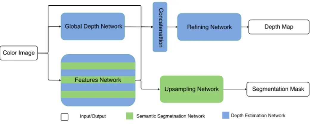
The lack of annotated RGB-D datasets, usually requires data augmentation tech-niques (i.e. flipping or cropping), in order to synthesize enough annotated data for training in supervised RGB-D segmentation. A different way to exploit depth in a supervised segmentation system is proposed in multi-task learning schemes [EF15, MPK16], in which the system is trained to jointly estimate the depth image and a segmentation mask for a color image. Since depth estimation and semantic segmenta-tion are two strongly correlated tasks, addressing them into unified approaches can be mutually beneficial. In this case, depth maps acquired from the depth sensor are used for training the system, in order to improve segmentation results even when depth will not be available at the testing stage.

(22)

1.2 Video Segmentation

A video formed as a sequence of images is usually employed in applications such as video surveillance and human motion analysis. Intuitively, video segmentation can be treated separately for each frame as a set of static image segmentation tasks. However, the spatial segmentation in each of the video frames is not always temporally consistent in the whole sequence due to the lack of necessary coherence constraints along the sequence. Therefore, it is worthwhile to consider temporal information in video segmentation straight from the start, instead of considering temporal coherence just as a constraint or as a post-processing issue.

Exploiting temporal information usually comes down to establishing the temporal correspondences between consecutive video frames. The correspondences can be es-tablished at different levels. For instance, Optical Flow techniques compute temporal correspondences at pixel level, estimating the pixel motion between to frames. Build-ing temporal correspondences at pixel level is a difficult task. For video segmentation purposes, often suffices to briefly represent local raw pixels at some higher scale and then refine this representation at each frame by analyzing temporal correspondences, in order to provide a temporally coherent segmentation.

In the following sub-sections, we first explain how the video frame representation problem is generally defined (Section 1.2.1). Then, we introduce the definition of building temporal correspondence based on the representations (Section 1.2.2). We also discuss how depth information can help in these two tasks.

1.2.1 Video Frame Representation

Representing video frames aims at grouping a large number of pixels into a small number of segments, while the object boundaries should be well preserved. In this manner, this brief representation of video frames simplifies the problem of building temporal correspondences. Representing video frames has a similar goal to the task of static image segmentation introduced in Section 1.1. In this case, more complex video frame representations such as hierarchical representation, generic object models

(23)

or object proposals are proposed in order to provide higher flexibility when building temporal correspondences. In the following subsections, we briefly review RGB based video frame representation methods, and explain how RGB-D data can help from this perspective.

RGB based Video Frame Representation

The introduction of a hierarchical representation allows establishing correspon-dences at different scales, which benefits the temporal coherence analysis. A hier-archical representation describes the raw data from coarse to fine, usually starting from segments at a relatively fine level generated by over-segmentation. Then, the segments are gradually grouped into coarser level regions.

Generic model-based representations describing objects in the scene with models such as surface model or Gaussian mixture model are employed to incrementally learn/update an object model along a sequence, which allows better tracking, or building temporal correspondences. But these object level representations still rely on a good initial configuration for the model. Since they are incrementally updated in each frame, they are also very sensitive to segmentation errors, which may accumulate over time.

Supervision is also usually exploited to represent a video frame. Apart from the su-pervision employed in static image segmentation methods, which can be leveraged to video frame representation, initialization may also serve as one special type of super-vision required in some tracking based video segmentation methods [RM07, TFNR12, PKB+_{17, CMPT}+_{17]. The advantage of introducing initialization is obvious, as it} provides clear targets/models for the system to perform robust segmentation in the following video frames. But it restricts these methods to certain types of application scenarios, where only a few foreground objects are of interest. Most computer vision applications involve large amounts of data with different types of scenes containing several objects, and this requires more genericity in video segmentation.

More recently, a representation based on object proposals [LKG11, ML12, ZJS13] have been introduced to represent raw data with a pool of object-like regions. These

(24)

‘object proposals’ are extracted from each frame based on generic spatial features. The advantage of these methods is that the extracted object proposals usually corresponds to object level segments. But to cover all the objects in the scene in the object proposal pool, redundant proposals are inevitably generated, which makes it computationally expensive.

Representation based on RBGD data

When RGB-D stream data is available, the added depth information makes more efficient to represent raw data in video frames. For instance, in hierarchical repre-sentations, depth information provides a better over-segmentation by considering the 3D spatial relations between pixels. It also helps defining a better grouping strategy when building the hierarchy. In generic model-based approaches, depth information provides the possibility to define the generic model in 3D rather than 2D. In repre-sentations based on object proposals, depth information, serving as an extra generic feature, helps on better generating the proposals. In supervised approaches, depth information provides an extra type of input sources so that richer features can be designed or learned in the training process to improve the performance of classifiers.

1.2.2 Building Temporal Correspondences

A video formed as a sequence of images also provides temporal information between elements in those images. Exploiting temporal coherence offers a way to segment video frames spatio-temporally. Temporal correspondences between video frames are built at different levels depending on the representation with varying difficulty at each level. The difficulty of building temporal correspondences varies depending on different levels. Temporal correspondences at the finest (pixel level) generated be-tween consecutive frames implicitly represent the optical flow of the two frames. In this case, the global optimum in the correspondence building task is still difficult to achieve considering the large scale of the problem. Instead, a local optimum is usually accepted as a solution for the correspondence problem, which makes the established

(25)

correspondences less reliable in subsequent analysis. On the other hand, building tem-poral correspondences at a coarser level reduces the scale of the problem, which allows to search for the global optimum in the correspondence building task. However, the segments at the coarser level between consecutive frames are not always temporally consistent, which may also lead to errors when building temporal correspondences.

When RGB-D stream data is available, the temporal correspondences between ob-jects in consecutive frames may show the actual movements/displacements of obob-jects in the real world 3D space. That is to say, building temporal correspondences for RGB-D stream data can be modeled based on a clear physical meaning. For instance, 3D displacements are more reliable than 2D displacements due to the fact that objects are captured at different scales on 2D images.

As explained in the previous sections, the emergence of depth data provides an-other source of data which can be applied in almost all aspects to better approach segmentation problems in computer vision. However, the problem of how to incorpo-rate efficiently depth information in segmentation tasks still needs further study.

1.3 Scope and Goals of This Dissertation

In this thesis, we aim to address different segmentation problems with RGB-D data. Despite the huge progress the field has experienced in the last few years, we consider there is still room for improvement. Since this dissertation has been per-formed in a period of fast changes in the state-of-the-art techniques, we investigate the way to efficiently incorporate depth information for both unsupervised segmenta-tion problems and supervised segmentasegmenta-tion problems.

Semantic segmentation is a core problem in the field of supervised image segmen-tation. With the successful application of Convolutional Neural Networks (CNNs) to semantic segmentation, a huge progress has been made in this field for RGB data. In this thesis, we first address the semantic segmentation problem by introducing depth information into state-of-the-art CNNs. We incorporate depth information in the training process of the CNN by following a multi-task learning framework.

(26)

Although CNNs based semantic segmentation methods achieve outstanding seg-mentation result due to the strong representation power of CNN, there are still some drawbacks which may limit its application for higher level applications. CNN based semantic segmentation restricts the approaches to several predefined semantics, while it usually requires a large amount of annotated data for training a classifier in order to obtain semantic labels at pixel level. Apart from that, semantic segmentation is also not aware of object instances, which makes it hard to apply to instance level applications. From the other perspective, most of the unsupervised image segmenta-tion approaches naturally have the advantage on coping with generic scenes. How-ever, object level segmentation can hardly be achieved in those approaches due to the lack of semantic information. To tackle these problems, we address an unsuper-vised generic instance segmentation problem based on RGB-D stream data, in which spatial-temporal information are analyzed based on generic features extracted from RGB-D data.

The performance of the generic instance segmentation method is highly restricted to the discriminative power of the employed hand-crafted features. On the other hand, CNNs based semantic segmentation methods introduce a good representation for the predefined semantics, which are trained to extract robust features via networks with a huge number of parameters. However, the cost of training those CNNs is not affordable in generic instance segmentation. In these situations, we propose a method to combine the genericity of generic instance segmentation and the strong representation power of CNNs by employing the idea of one shot learning which learns an object model based on one (or very few) example of an object discovered in a sequence.

Our work and contributions are divided into three main parts listed hereafter:

Part I: Semantic Segmentation based on RGB-D Data

In this part, we address the problem of how to incorporate depth information in a CNN based semantic segmentation task.

Our contributions are:

(27)

se-mantic segmentation, in which both tasks benefit from each other in the hybrid architecture

• We clarify how the two tasks help each other in a hybrid system by investigat-ing the common attributes as well as the distinction in depth estimation and semantic segmentation

• The hybrid architecture is verified and applied in different scenarios

Part II: Generic Instance Segmentation based on RGB-D Stream Data

Semantic segmentation is restricted to a few predefined types of semantics, which can be hardly applied to more generic scenes, such as when undefined new objects move into the scene. On the other hand, semantic segmentation is not aware of individual object instances. This also compromises the application of semantic seg-mentation for applications such as interaction analysis and instance counting. In this part, we propose an unsupervised instance segmentation approach based only on generic features extracted from RGB-D stream data.

• A novel hierarchical representation for the 3D point cloud of a scene, which allows to establish temporal correspondences efficiently at different scales of object-connectivity

• An approach to tackle the temporal correspondence problem. The proposed approach converts the problem to a labels assignment task, and solves it with an optimization method

• A mechanism to deal with possible object splits and merges along time. It maintains the similarities between nodes in the hierarchy in order to deal with possible object splits and merges.

Part III: One-Shot Learning for Generic Instance Segmentation based on RGB-D stream data

(28)

Generic features employed in generic segmentation methods have limited discrim-inative power to distinguish different objects in the scene, while CNN based semantic segmentation is restricted to predefined semantics and not aware of object instances. In this part, we combine the advantages of the two methods, that is the strong ob-ject representation power of CNNs and the genericity of the unsupervised instance segmentation method, and apply the combined approach to solve a generic instance segmentation problem in RGB-D video sequences.

• A one-shot learning approach, allowing to represent the appearance of an object instance when it is discovered by the generic instance segmentation method

1.4 Organization of The Thesis

Specific contributions of this thesis mentioned in the three parts above are dis-cussed in each corresponding Chapter (3, 4, and 5) after the relevant state-of-the-art (Chapter 2). The conclusions in Chapter 6 summarize the contributions, and also include a list of journal papers, international conference publications, contributions to projects and submitted publications as a result of the work in this thesis. The basic knowledge related to the thesis is included in the appendices. The organization of this thesis is, thus, as follows:

Chapter 1Introduction to the thesis subject, the background of this subject and

the organization of this thesis.

Chapter 2An overview of the relevant state-of-the-art publications and methods

related to semantic segmentation and generic segmentation.

Chapter 3 (Part I): Semantic Segmentation based on RGB-D data Chapter 4 (Part II): Generic Instance Segmentation based on RGB-D Stream Data

Chapter 5 (Part III): One-Shot Learning for Generic Instance

Segmen-tation based on RGB-D stream data, where classical generic segmentation and

(29)

Chapter 6: Conclusions and Future Work The final conclusions, contribu-tions, related publications and future work are included in this chapter.

Appendix AThe fundamentals of Convolutional Neural Network related to this

thesis.

Appendix B The fundamentals of Conditional Random Field related to this

(30)

Chapter

2

State of the Art

Segmentation is a classical topic in computer vision. The computer vision commu-nity has produced an increasing number of contributions to address this problem in recent years. Traditionally, the segmentation techniques were developed based mainly on photometric information in color images. The recent emergence of consumer depth sensors provides the opportunity to incorporate geometric information in the segmen-tation process coping with problems that could hardly be addressed only based on photometric data, such as scale changes, lighting conditions and background clutter. Following the taxonomy introduced in Chap 1, we have categorized segmentation problems into RGB/RGB-D based segmentation, unsupervised/supervised segmen-tation and image/video segmensegmen-tation. In this thesis, we aim at solving different segmentation problems with RGB-D data. Specifically, we start with a semantic im-age segmentation problem, which is core in supervised segmentation. We study the current background of approaches tackling semantic segmentation problems in Sec-tion 2.1. Complementary to semantic segmentaSec-tion, unsupervised image segmentaSec-tion systems can be applied in more general applications where the semantics cannot be predefined, or instance level segmentation is needed. We review these approaches in Section 2.2. Unsupervised approaches mainly focus on generating spatially coherent segments and can hardly produce segments at object level due to the lack of infor-mation in a single image. However, they provide a good image representation for further analysis when more information is available, such as temporal information

(31)

in video sequences. Exploiting temporal information may help in achieving object level segmentation in unsupervised approaches. Thus, we study video segmentation approaches in the state-of-the-art by reviewing methods exploiting temporal infor-mation in Section 2.3. In each category, we first review RGB based methods in the state-of-the-art, then explain how depth information helps when these methods are extended to deal with RGB-D, so that we study the contribution of RGB-D data in different segmentation problems.

2.1 Semantic Segmentation

Semantic segmentation is a task of recognizing and understanding object classes at the pixel level. It follows the schema of recognition, in which pixels are first represented by features, then classified into different object classes. In the following subsections, we will first review the traditional semantic segmentation techniques, then we study the more up-to-date Convolutional Neural Networks (CNNs) for semantic segmentation. Under each branch, we review both RGB and RGB-D based approaches to study how RGB-D data helps in different situations.

2.1.1 Traditional Semantic Segmentation

Traditionally, semantic segmentation is done with a classifier which operates on fixed-size feature inputs and a sliding-window approach. The classifier is usually trained on features extracted from image patches with a fixed size. In the test phase, the trained classifier is fed with features extracted from rectangular regions of an image, which are called windows. The center pixel is classified according to the information contained in the window. Sliding the window and classifying its features produces the labels for all pixels on the image. The two main problems in classical semantic segmentation approaches are: 1) pixel description, in which we study how to represent a pixel on the image with features in order to train the classifier efficiently, 2) training techniques, in which we study methods used to train a classifier based on

(32)

the extracted features.

RGB based Pixel Description

The choice of features is very important in traditional approaches. In this section, we review the most commonly used features in a semantic segmentation task.

Pixel Color: Pixel color is the most widely used feature. Pixel color is described

in different color spaces, providing different representations. Typically the colors of pixels in an image are represented in the RGB color space. No single color space has been proven to be superior to all others in all contexts [CJSW01]. However, the most common choices seem to be RGB and color spaces based on luminance and color.

Histogram of Oriented Gradient: The original image is transformed into two

feature maps of equal size which represent the gradient, that is, the partial derivative in x and y for each pixel. These feature maps are split into patches and a histogram of the directions is calculated for each patch. HOG features were proposed in [DT05] and are widely used for segmentation tasks [BMBM10, FGMR10].

Scale Invariant Feature Transform (SIFT): SIFT descriptors [Low04]

repre-sent key-points in an image. An image patch of size 16×16 around the key-point is taken. This patch is divided in 16 distinct parts of size 4×4. For each of those parts a histogram of 8 orientations is calculated similar as for HOG features. This results in a 128-dimensional feature vector for each key-point. In [PTN09], Plath et al. use SIFT to describe image patches at different scales and train the classifier on patch features using a Support Vector Machine (SVM) to produce semantic labeling.

Bag of Visual Words (BOV): BOV is based on vector quantization. Similar

to HOG features, BOV features are histograms that count the number of occurrences of certain patterns within a patch of the image [CDF+_{04]. In [CP08], Csurka et} al. use BOV to transform the low level features into a high level representation. A Gaussian Mixtured Model (GMM) is employed to model the visual vocabulary of the low level features, in which each Gaussian corresponds to a visual word. These high level features are then used for semantic segmentation.

(33)

RGB-D based Pixel Description

Consumer depth sensors produce a depth map registered with a color image, where distance information of the scene to the camera is stored pixel-wise. In the case of feature extraction on a depth map, a straightforward way is to extend the existing methods for color and apply them to depth maps. For instance, Histogram of Oriented Depth (HOD) [SA11] is proposed similarly to HOG, in which a histogram of the orientation of the depth gradient is calculated for patches on a depth map. Besides, a 3D point cloud can be back-projected from a depth map by transforming the per-pixel distances using the camera parameters. The 3D point cloud represents discrete points of the surface of the scene from the viewpoint of the camera, with rich geometric information. Several 3D features extracted from 3D point clouds are proposed.

3D Coordinates: 3D coordinates of a point on a point cloud represents its spatial

localization in the real world 3D space. The similarity between 3D coordinates of different points shows their physical spatial relationship.

3D Normals: 3D normals are important features of a geometric surface, and

are also used to create higher level 3D features. Given a geometric surface, it is usually trivial to infer the direction of the normal at a certain point by estimating the vector perpendicular to the surface at that point. Since the point cloud acquired from consumer depth sensors represents a set of points sampled on the real surface, there are usually two ways to approximate the surface normal of a point:

• obtaining the underlying surface from the point cloud, using surface meshing techniques, and then compute the surface normals from the mesh

• using approximations to infer the surface normals from the point cloud directly For instance, in [Rus09], estimating the surface normal is reduced to an analysis of the eigenvectors and eigenvalues of a co-variance matrix created from the nearest neighbors of the query point on the point cloud.

Point Feature Histogram (PFH)/Fast Point Feature Histograms (FPFH):

The idea of the PFH [Rus09] is to encode the geometrical properties of thek-neighborhood of a point by generalizing the mean curvature around the point from a multi-dimensional

(34)

histogram of values. This highly dimensional hyperspace provides an informative sig-nature for the feature representation, is invariant to the 6D pose of the underlying surface, and copes very well with different sampling densities or noise levels present in the neighborhood. A Point Feature Histogram representation is based on the rela-tionship among the points in thek-neighborhood and their estimated surface normals. Due to the high computational complexity of PFH, a simplification called FPFH [Rus09] is proposed. In FPFH, the feature computing is just performed between the query point and its neighbors, rather than each pair of points within its neighborhood. FPFH is used as a local shape feature in the segmentation task in [PASW13].

Spin Image: The spin image is a surface representation technique that was

in-troduced in [Joh97]. Spin images encode the global properties of any surface in an object-oriented coordinate system rather than in a viewer-oriented coordinate system. By using object-oriented coordinate systems, the description of a surface or an object is view-independent and it does not change as the viewpoint changes. Given a 3D point and its normal, it represents the distribution of the projections of all points on the point cloud to the tangent plane of the query point. In [MKRVG15], spin image is used as a feature for a semantic segmentation task.

Training Techniques

In a semantic segmentation task, a classifier is usually trained based on the ex-tracted features in order to obtain semantic labels for each pixel in the test phase.

Support Vector Machine (SVM): Originally, SVM [CV95] was proposed for

linear two-class classification with margin, where margin means the minimal distance from the separating hyper-plane to the closest data points. SVM seeks for an optimal separating hyper-plane, where the margin is maximal. An important and unique feature of this approach is that the solution is based only on those data points, which are at the margin. These points are called support vectors. The linear SVM can be extended to a nonlinear one when the feature space is first transformed using a set of nonlinear basis functions. In this feature space, which can be very high dimensional, the data points can be separated linearly. An important advantage of

(35)

SVM is that it is not necessary to implement this transformation and to determine the separating hyper-plane in the possibly very-high dimensional feature space, instead a kernel representation can be used, where the solution is written as a weighted sum of the values of a certain kernel function evaluated at the support vectors. As an example, SVMs are used to train the classifier [YHRF12] for a semantic segmentation task.

Random Forest: Random Forests were first proposed in [Ho95]. This type

of classifier applies techniques called ensemble learning, where multiple classifiers are trained and a combination of their hypotheses is used. In the case of Random Forests, the classifiers are decision trees. A decision tree is a tree where each inner node uses one or more features to decide in which branch to descend, and each leaf represents a class. One strength of Random Forests compared to many other classifiers like SVMs and neural networks is that the scale of measure of the features (nominal, ordinal, interval, ratio) can be arbitrary. Random Forests are applied to train the classifier in [SJC08] for segmentation.

2.1.2 Convolutional Neural Networks based Semantic

Seg-mentation

Traditional semantic segmentation methods are usually restricted to the limited discriminative power of hand-crafted pixel features. To overcome the limitation of the hand-crafted features, Convolutional Neural Networks (CNNs) were proposed to learn feature extractors from a set of training data. A CNN can be interpreted as the combination of a set of feature extractors and a classifier, where we train the network to extract better features and classify them into different classes. The classification errors of the training samples are back-propagated to update the parameters of the network, while the classification error is optimized. CNNs were first applied in an im-age classification task [KSH12], in which a deep network with millions of parameters was trained on large scale datasets, in order to learn robust feature extractors for clas-sifying images. As with outstanding achievements in CNNs based image classification,

(36)

CNNs have also had enormous success on segmentation problems.

One of the popular initial CNNs based approaches was patch classification where each pixel was separately classified into classes using a patch of image around it. The main reason to use patches was that classification networks usually have fully connected layers and therefore required fixed size images.

In 2015, Fully Convolutional Network (FCN) [LSD15] by Long et al. popularized CNN architectures for dense predictions without any fully connected layers. This allowed segmentation maps to be generated for images of any size and was also much faster compared to the patch classification approach. Almost all the subsequent state-of-the-art approaches on semantic segmentation adopted this paradigm.

Apart from fully connected layers, one of the main problems of using CNNs for segmentation are the pooling layers. Pooling layers increase the field of view and are able to aggregate the context while discarding the “where” information. However, semantic segmentation requires the exact alignment of class maps and thus, needs the ‘where’ information to be preserved. Two different classes of architectures evolved in the literature to tackle this issue.

The first one is the encoder-decoder architecture. Encoder gradually reduces the spatial dimension with pooling layers and decoder gradually recovers the object de-tails and spatial dimension. There are usually shortcut connections from encoder to decoder to help the decoder recover the object details better. U-Net [RFB15] is a pop-ular architecture from this class. It consists of a contracting path to capture context in the encoder and a symmetric expanding path from the encoder layers to the decoder layers that enables precise localization. Seg-Net [BKC17] is proposed based on FCN. It introduces more shortcut connections between encoder and decoder. Furthermore, it copies the indices from the max-pooling layers in the encoder to the decoder instead of copying the encoder features as in FCN, which makes easier for SegNet to recover the spatial information and is more memory efficient than FCN.

Architectures in the second class use what are called dilated/atrous convolutions [YK16, CPK+_{16]. Pooling layers help in classification networks because they increase} the receptive field of a network. But, as mentioned, this is not suitable for a

(37)

seman-tic segmentation task, since pooling drops the spatial information and decreases the resolution. Atrous/Dilated convolutions can compute responses at all image positions with an n times larger receptive field if the full resolution image is convolved with a filter ‘with holes’, in which the original filter is upsampled by a factorn, and zeros are introduced in between filter values. Although the effective filter size increases, it is only necessary to take into account the non-zero filter values, hence both the number of filter parameters and the number of operations per position stay constant.

CNNs based Semantic Segmentation using RGB-D data

CNNs based segmentation approaches require a large mount of annotated data, which makes its application to RGB-D data difficult, due to the lack of annotations in RGB-D datasets. Nevertheless, there are approaches that directly encode the depth map as an extra input for training the networks. In this case, CNNs may benefit from the richer information input. For instance, [GGAM14] proposes to incorporate the depth map encoded as a pixel feature map in the training process of a CNN architecture. However, data augmentation, such as flipping, cropping etc, plays an important role in these approaches.

Another way to take advantage of the depth information in a CNNs based se-mantic segmentation approach is to follow a multi-task learning scheme, in which depth estimation and semantic segmentation are tackled in a hybrid CNN architec-ture. Since depth estimation and semantic segmentation are two strongly correlated tasks, addressing them into unified approaches can be mutually beneficial. In this case, the feature extractors in the hybrid network are better trained to cope with both semantic segmentation and depth estimation, which implicitly incorporates the depth information in CNNs.

These hybrid networks are usually designed as a combination of networks working for a single task. It is worthwhile to first study representative single task based ap-proaches before reviewing apap-proaches under multi-task learning schemes. In Section 2.1.2, we have studied the state-of-the-art CNNs based semantic segmentation ap-proaches. In the following paragraphs, we first review CNNs based depth estimation

(38)

approaches, then address the multi-task based approaches in the state-of-the-art. For the task of CNNs based depth estimation from monocular images, one of the first efforts was made by Eigen et al in [EPF14]. This approach estimates a low resolu-tion depth map from an input image as a first step, then finer details are incorporated by a fine-scale network that locally refines the low resolution depth map using the in-put image as a reference. Additionally, the authors introduced a scale-invariant error function that measures depth relations instead of scale. Ivaneck´y [Iva16] presents an approach inspired in [EPF14], incorporating estimated gradient information to im-prove the fine tuning stage. Additionally, this work applies a normalized loss function leading to an improvement in depth estimation.

On the other hand, approaches addressing depth estimation and semantic seg-mentation with multi-task learning schemes currently receive large attention due to its potential of improving the performance in multiple tasks. In [WSL+15] a unified framework was proposed that incorporates global and local prediction under an archi-tecture that learns the consistency between depth and semantic segmentation through a joint training process. Another unified framework is presented in [EF15] where depth map, surface normals and semantic labeling are estimated. The results obtained by [EF15] outperformed the ones presented in [EPF14] proving how the integration of multiple tasks into a common framework may lead to a better performance of the tasks. A more recent multi-task approach is introduced in [MPK16]. The methodol-ogy proposed in this work makes initial estimations for depth and semantic label at a pixel level through a joint network. Later, depth estimation is used to solve possible confusions between similar semantic categories and thus to obtain the final semantic segmentation. Another multi-task approach by Teichmann et al. [TWZ+_{16] presents} a network architecture named MultiNet that can perform classification, semantic seg-mentation and detection simultaneously. They incorporate these three tasks into a unified encoder-decoder network where the encoder stage is shared among all tasks and specific decoders for each task producing outputs in real-time. This work efforts were focused on improving the computational efficiency for real-time applications as autonomous driving. A similar approach is Pixel Level Enconding and Depth

(39)

Layer-ing (PLEDL) [UCFB16], which extended FCN [LSD15] with three output channels jointly trained to obtain pixel-level semantic labeling, instance-level segmentation and 3D depth estimation.

2.2 Unsupervised Segmentation

Different from semantic segmentation approaches, where a group of semantics can be predefined before solving the segmentation problem, unsupervised segmentation approaches aim at tackling image segmentation problems in more general scenarios. While semantic segmentation approaches store information about the semantics they were trained to segment under the supervision of training data, unsupervised segmen-tation approaches try to detect consistent regions or region boundaries with respect to generic features. Although unsupervised segmentation approaches can hardly be semantic, they still provide generic representations of an image, which can be used in supervised segmentation as another source of information or to refine a segmen-tation when more information, such as temporal information in videos, is available. Since unsupervised segmentation problems are well-studied in recent decades, a large amount of approaches were proposed. We review some of the most representative unsupervised approaches as follows:

2.2.1 Clustering Algorithms

Clustering algorithms can directly be applied on the pixels, when one gives a feature vector per pixel. Two famous clustering algorithms arek-means and the mean-shift algorithm. The k-means algorithm is a general-purpose clustering algorithm which requires the number of clusters to be given beforehand. Initially, it places the

k centroids randomly in the feature space. Then it assigns each data point to the nearest centroid, moves the centroid to the center of the cluster and continues the process until a stopping criterion is reached. A faster variant is described in [HH75]. k-means was applied by [CLP98] for medical image segmentation.

(40)

Another clustering algorithm is the mean-shift algorithm which was introduced by [CM02] for segmentation tasks. The algorithm finds the cluster centers in a feature space by initializing centroids at random seed points and iteratively shifting them to the mean position in the feature space within a certain range. Instead of taking a hard range constraint, the mean can also be calculated by using any kernel. This effectively applies a weight to the coordinates of the points. The mean shift algorithm finds cluster centers at positions with a highest local density of points.

2.2.2 Watershed Segmentation

The watershed algorithm takes a feature, such as the gradient magnitude, from a grayscale image and interprets it as a height map. Low values are catchment basins and the higher values between two neighboring catchment basins form the watershed lines. In order to detect the homogeneous regions of an image, the watershed is usually applied on a variational feature on the image. The algorithm starts to fill the basins from the lowest point. When two basins are connected, a watershed is found. The algorithm stops when the highest point is reached. A detailed description of the watershed segmentation algorithm is given in [RM00]. An as example, the watershed segmentation was used in [JLD03] to segment white blood cells. As the authors describe, the segmentation by watershed transform has two flaws: Over-segmentation due to local minima and thick watersheds due to plateaus.

2.2.3 Active Contour Models

Active contour models (ACMs) are algorithms that segment images roughly along edges, but also try to find a border which is smooth. This is done by the minimization of an energy function computed on the resulting contour. They were initially described in [KWT88]. ACMs can be used to segment an image or to refine segmentation as it was done in [AM98] for brain MR images.

(41)

2.2.4 Graph based Segmentation

Graph-based image segmentation algorithms typically interpret pixels as vertices and an edge weight is a measure of dissimilarity, such as the difference in color [FH04]. In this case, there are several different candidates for edges, such as the 4-neighborhood or an 8-neighborhood.

In graph based approaches, a segmentation is a partition of the vertex set into segments, where each segment corresponds to a connected component in the graph. Graph based approaches obtain a segmentation by removing edges connecting vertices, while producing non-connected sub-graphs (segments). One intuitive way to cut the edges is by first building a minimum spanning tree of the graph, then removing edges on the minimum spanning tree above a threshold [Zah71] to obtain the segments. This threshold can either be constant, adapted to the graph or adjusted by the user. After the edge-cutting step, the connected components are the segments. However, since differences between pixels within high variability regions can be larger than those between the ramp and the constant regions, it is difficult to find an adequate threshold. In [FH04], the authors propose a more efficient way to approach the graph based image segmentation problem, in which pixels are iteratively merged into segments by comparing the internal difference of a segment (measured by the maximum edge weight within the minimum spanning tree of the segment) and the difference between segments (represented by the minimum edge weight connecting the two segments).

Another way to perform graph based image segmentation is based on cutting the edges with minimum weights in a graph, where the cut criterion is designed to minimize the similarity between vertices on the graph that are being split. This problem is solved by graph cut algorithms, such as Stoer and Wanger algorithm [SW97], Ford-Fulkerson algorithm [FF56], etc. The work in [WL93] introduces such a cut criterion for image segmentation purposes. However, it is biased towards finding small segments. In [SM00], the bias is addressed with the normalized cut criterion, which takes into account both the total dissimilarity between the different segments as well as the total similarity within each segment.

(42)

pixels leads to a large scale problem of graph based image segmentation. Additionally, the graph constructed directly from pixels is also very sensitive to the pixel noise. In this case, a prior pixel grouping step is usually introduced to abstract pixels into locally homogeneous patches, called super-pixels. For instance, the work in [ASS+_12] proposes a Simple Linear Iterative Clustering (SLIC) method, which adapts a k-means clustering approach to efficiently generate super-pixels. In [CM02], mean shift is applied to find modes (super-pixels) in a color or intensity feature space. The adjacency graph of the obtained super-pixels is usually employed in graph based image segmentation approaches, in order to reduce the number of vertices and edges in the graph while preserving important boundary information.

2.2.5 RGB-D based Unsupervised Segmentation

Similar to RGB-D based supervised approaches, RGB-D based unsupervised ap-proaches extended from RGB methods, and usually add depth values as an extra feature of the data, such as [WGB12]. Apart from that, there are also methods work-ing with 3D point clouds instead of depth values. For instance, [CSSPW14] begins by decomposing the 3D point cloud of the scene into an adjacency-graph of surface patches based on a voxel grid. Edges in the graph are then classified as either convex or concave using a novel combination of simple criteria which operate on the local geometry of these patches. In this way, the graph is divided into locally convex con-nected sub-graphs, which with high accuracy represent object parts. In [PASW13], Papon et al. propose a novel unsupervised over-segmentation approach that uses voxel relationships to produce over-segmentations, which are fully consistent with the spatial geometry of the scene in three dimensional, rather than projective space. Enforcing the constraint that segmented regions must have 3D spatial connectivity prevents super-voxels from flowing across object boundaries.

Semantic and generic object segmentation for scene analysis using RGB-D Data

Semantic and generic object segmentation

for scene analysis using RGB-D data

by Xiao Lin

Universitat Polit`

ecnica de Catalunya

Departamento de Teoria del Senyal i Comunicacions

Semantic and Generic Object Segmentation for

Scene Analysis Using RGB-D Data

by

Xiao Lin

Doctoral Thesis

Advisors: Josep Ramon Casas and Montse Pard`

as

Abstract

Acknowledgments

Contents

List of Figures

Acronyms

Chapter

1

Introduction and Overview

1.1

Static Image Segmentation

1.1.1

RGB based Image Segmentation

1.1.2

RGB-D based Image Segmentation

1.2

Video Segmentation

1.2.1

Video Frame Representation

1.2.2

Building Temporal Correspondences

1.3

Scope and Goals of This Dissertation

1.4

Organization of The Thesis

Chapter

2

State of the Art

2.1

Semantic Segmentation

2.1.1

Traditional Semantic Segmentation

2.1.2

Convolutional Neural Networks based Semantic

Seg-mentation

2.2

Unsupervised Segmentation

2.2.1

Clustering Algorithms

2.2.2

Watershed Segmentation

2.2.3

Active Contour Models

2.2.4

Graph based Segmentation

2.2.5

RGB-D based Unsupervised Segmentation

_{Xiao Lin}