FULL PAPER
Should tsunami simulations include a
nonzero initial horizontal velocity?
Gabriel C. Lotto
1*, Gabriel Nava
1,3and Eric M. Dunham
1,2Abstract
Tsunami propagation in the open ocean is most commonly modeled by solving the shallow water wave equations. These equations require initial conditions on sea surface height and depth-averaged horizontal particle velocity or, equivalently, horizontal momentum. While most modelers assume that initial velocity is zero, Y.T. Song and collabo-rators have argued for nonzero initial velocity, claiming that horizontal displacement of a sloping seafloor imparts significant horizontal momentum to the ocean. They show examples in which this effect increases the resulting tsunami height by a factor of two or more relative to models in which initial velocity is zero. We test this claim with a “full-physics” integrated dynamic rupture and tsunami model that couples the elastic response of the Earth to the linearized acoustic-gravitational response of a compressible ocean with gravity; the model self-consistently accounts for seismic waves in the solid Earth, acoustic waves in the ocean, and tsunamis (with dispersion at short wavelengths). Full-physics simulations of subduction zone megathrust ruptures and tsunamis in geometries with a sloping seafloor confirm that substantial horizontal momentum is imparted to the ocean. However, almost all of that initial momen-tum is carried away by ocean acoustic waves, with negligible momenmomen-tum imparted to the tsunami. We also compare tsunami propagation in each simulation to that predicted by an equivalent shallow water wave simulation with vary-ing assumptions regardvary-ing initial velocity. We find that the initial horizontal velocity conditions proposed by Song and collaborators consistently overestimate the tsunami amplitude and predict an inconsistent wave profile. Finally, we determine tsunami initial conditions that are rigorously consistent with our full-physics simulations by isolating the tsunami waves from ocean acoustic and seismic waves at some final time, and backpropagating the tsunami waves to their initial state by solving the adjoint problem. The resulting initial conditions have negligible horizontal velocity. Keywords: Tsunami, Tsunami modeling, Tsunami generation, Offshore earthquake, Subduction zone, Shallow water wave equations
© The Author(s) 2017. This article is distributed under the terms of the Creative Commons Attribution 4.0 International License (http://creativecommons.org/licenses/by/4.0/), which permits unrestricted use, distribution, and reproduction in any medium, provided you give appropriate credit to the original author(s) and the source, provide a link to the Creative Commons license, and indicate if changes were made.
Introduction
Tsunamis from earthquake sources pose a significant threat to coastlines around the world and have killed hundreds of thousands of people in the last few decades. The Earth science community often relies on numerical models to better understand tsunami physics (e.g., Titov and Synolakis 1998; Tanioka and Satake 1996; Kowalik
2003), perform hazard assessments (e.g., Geist and Par-sons 2006; Borrero et al. 2006; González et al. 2009), and plan for early warning (e.g., Titov et al. 2005; Melgar and Bock 2013; Behrens et al. 2010).
For numerical modelers, the tsunami life cycle is often divided into three parts: generation, propagation, and inundation (Bernard et al. 2006; Mori et al. 2011; Titov and Gonzalez 1997; Watts et al. 2003; Song and Han 2011). This paper is entirely focused on the first two parts, though modeling inundation poses its own unique set of chal-lenges and is far from being completely understood.
It is fairly straightforward to model tsunami propaga-tion in the open ocean, as reviewed by Satake (2002). The simplest and most common way to do so is by using the linearized shallow water wave equations, based on assumptions of inviscid, incompressible water; small amplitude waves; and horizontal wavelengths greater than the ocean depth. In one horizontal dimension, the equations are
Open Access
*Correspondence: [email protected]
1 Department of Geophysics, Stanford University, Stanford, CA, USA
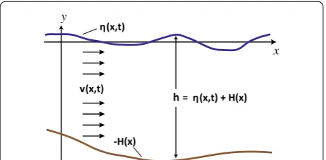
Here, x and y the horizontal and vertical spatial coordi-nates, respectively, t is time, h=h(x,t) is the depth of the ocean, v=v(x,t) is the depth-averaged horizontal veloc-ity, and g is the gravitational acceleration. As in Fig. 1, we define the sea surface perturbation about y=0 as
y=η(x,t) and the position of the seafloor as y= −H(x) , so that h(x,t)=η(x,t)+H(x). Linearization is justified
assuming |η(x,t)| ≪ |H(x)|. The equations describe
non-dispersive wave propagation at speed √gH.
Time-dependent seafloor displacement, which gener-ates the tsunami, can be accounted for through an addi-tional term in the mass balance Eq. (1). However, it is more common to account for seafloor displacement indi-rectly through initial conditions. This is justified when the tsunami propagation distance over the rupture dura-tion is much smaller than horizontal scales of interest. This condition is almost always satisfied because earth-quake ruptures propagate at elastic wave speeds that are an order of magnitude faster than the tsunami propaga-tion speed (Kajiura 1970).
Solving Eqs. (1) and (2) requires two initial conditions,
These initial conditions are, of course, determined by the tsunami generation process. For a tsunami generated by an undersea earthquake on an initially flat seafloor (i.e., H(x)=constant), the simplest choice for η0(x) is to
assume that the vertical static displacement of the sea-floor following the earthquake, uy(x), is mirrored at the
sea surface, so that
(1) ∂η
∂t +
∂(Hv) ∂x =0,
(2)
∂v
∂t +g
∂η ∂x =0.
(3) η(x, 0)=η0(x),
(4) v(x, 0)=v0(x).
A more nuanced approach involves filtering out short wavelength variations to account for the nonhydrostatic ocean response at horizontal wavelengths smaller than H when translating the seafloor uplift to the sea surface (Kajiura 1963; Saito and Furumura 2009; Saito 2013).
If the seafloor is not flat, horizontal displacements also uplift the sea surface, as recognized by Tanioka and Satake (1996). For horizontal displacement ux along a seafloor with slope dH/dx, the contribution to η0(x) from
horizon-tal displacements is uxdH/dx, and thus the appropriate initial condition on sea surface displacement is
Because subduction zone plate boundary faults tend to dip at shallow angles of ∼10◦, ux is often significantly larger than uy, making the contribution from horizontal seafloor
displacement significant even for gently sloping continen-tal shelves. The role of horizoncontinen-tal seafloor displacement, as described by Tanioka and Satake, has gained widespread acceptance in the tsunami modeling community, and Eq. (6) has been widely used to match tsunami data and to make probabilistic estimates of tsunami hazard (e.g., Fujii et al. 2011; Geist and Parsons 2006; Sato et al. 2011).
With regard to initial velocity, the standard approach assumes that the initial depth-averaged horizontal veloc-ity is negligible, i.e.,
This assumption is exactly correct for an inviscid ocean with a flat seafloor (e.g., Saito 2013) since in that case shear traction vanishes at the seafloor and the normal traction there is exactly vertical. But it is not immediately obvious that the initial horizontal velocity should be zero when the seafloor is sloping and is displaced horizontally. In this case, normal traction on the seafloor has a hori-zontal component that will impart horihori-zontal momen-tum from the solid Earth to the ocean. This momenmomen-tum exchange will certainly occur, as pointed out by Song et al. (2008) based on the impulse-momentum theory, but the relevant question is whether this momentum plays a non-negligible role in tsunami generation. In a compressible ocean, it is also possible for this momentum to be carried away from the source region by ocean acoustic waves.
We briefly note an important consequence of choos-ing a nonzero value for v0(x), which might be testable
with tsunami waveform observations if there is suffi-cient uniqueness in the solution of the inverse problem of determining initial conditions from data. A nonzero initial velocity introduces asymmetries in the sea surface profile as the tsunami propagates, as illustrated by the (5) η0(x)=uy(x).
(6) η0(x)=uy(x)+ux
dH
dx.
(7) v0(x)=0.
x y
h = η(x,t) + H(x) η(x,t)
-H(x) v(x,t)
simple example shown in Fig. 2. A tsunami model with an initial condition other that (7) must justify this asym-metry. To the best of our knowledge, this asymmetry is not seen in tsunami observations, though it might be challenging to detect if the initial v0(x) is rather small and
bathymetric effects complicate the tsunami waveform. We return to this point subsequently.
In recent years, Song et al. (2008, 2017), Song and Han (2011), Titov et al. (2016), and Xu and Song (2013) have
our previous understanding of tsunami generation. The theory therefore merits a thorough investigation.
Drawing from impulse-momentum theory, Song et al. propose that the force exerted by the moving seafloor slope on the ocean transfers horizontal momentum to the ocean. They capture this effect in an approximate manner by estimating the accelerated horizontal particle velocity �v(x,y) of water in an incompressible ocean in
the vicinity of a moving slope as
0 100 200 300 400 500 600 700 800
horizontal distance (km) -5
0 5 10
amplitude (m
)
t = 0 s
0 100 200 300 400 500 600 700 800
horizontal distance (km) -5
0 5 10
amplitude (m
)
t = 700 s
0 100 200 300 400 500 600 700 800
horizontal distance (km) -0.4
-0.2 0 0.2 0.4
horiz. velocity (m/s
)
t = 0 s
0 100 200 300 400 500 600 700 800
horizontal distance (km) -0.4
-0.2 0 0.2 0.4
horiz. velocity (m/s
)
t = 700 s a
c
b
d
symmetric asymmetric
Fig. 2 Snapshots from a shallow water wave model for wave height η(x,t) (a) and (b) and horizontal velocity v(x,t) (c) and (d). The blue and red
simulations both have the same initial condition on η0(x), as in (a), and both have oceans with constant 4 km depth. Blue has v0(x)=0 and red
has v0(x)�=0, as seen in (c). The nonzero initial condition on horizontal velocity leads to a tsunami with an asymmetric sea surface profile, whereas
v0(x)=0 produces a symmetric tsunami for an ocean of constant depth
promoted an alternative theory of tsunami generation that includes, in addition to the processes encapsulated by Eq. (6), an additional horizontal momentum transfer from the solid Earth to tsunamis in the ocean that leads to non-negligible initial velocity v0(x). They suggest that
this momentum transfer increases the kinetic energy of the ocean and substantially contributes to tsunami wave heights. For example, they claim this effect accounts for two-thirds of the height of the 2004 Indian Ocean tsu-nami (Song et al. 2008) and half of the 2011 Tohoku, Japan, tsunami (Xu and Song 2013). If the Song et al. the-ory is correct and its effect on tsunami height is of the magnitude they claim, it would highlight a major gap in
(8)
�v(x,y)=
ux(x)/τ, −H(x)≤y≤ −Rx
0, otherwise , Rx=H(x)−min
H(x),LH dH
dx
where τ ∼ 5–20 s is the rise time, and LH is the effective
range of horizontal motion (Xu and Song 2013; Titov et al. 2016; Song et al. 2017). In more than one publica-tion, Song and Han (2011) and Xu and Song (2013) have used LH =1.5Hmax, where Hmax is the maximum depth
of the ocean. However, Song et al. (2017) have recently suggested that a position-dependent effective range,
LH =0.5H(x), might be more appropriate. The choice of LH has a large impact on the amplitude of tsunami waves,
and so we examine both versions of LH in this study. The
In this paper, we rigorously test the tsunami generation theory of Song et al. by running several “full-physics” earthquake and tsunami models (details provided subse-quently) and comparing them to the results of a simple shallow water model. By varying the initial horizontal velocity condition of the shallow water model, we can determine whether or not the initial condition described by Song et al. provides an accurate match to tsunami waveforms in the more realistic full-physics model.
Modeling approach
As mentioned above, we perform two parallel sets of tsu-nami simulations, one with a depth-resolved, coupled solid Earth-ocean model and the other with a depth-aver-aged shallow water wave model.
The fully-coupled, or full-physics, model is a 2-D depth-resolved model introduced by Lotto and Dunham (2015), building on earlier work by Maeda and Furumura (2013). We solve the elastic wave equation in the solid Earth and the acoustic wave equation in the compressible, inviscid ocean, and incorporate gravity via a modified free sur-face boundary condition. Small wave amplitudes, relative to ocean depth, are assumed to justify a linearization of the free surface condition. However, no assumption is made regarding horizontal wavelengths relative to ocean depth; the ocean response becomes nonhydrostatic at short wavelengths, giving rise to well-known effects such as the filtering of short wavelength features in the initial sea surface height and dispersion during tsunami propa-gation (Kajiura 1963, 1970). In the full-physics model, the earthquake source and all waves are simultaneously gen-erated, unlike the typical approach of first modeling the earthquake and then using the final displacement from the earthquake model to set initial conditions for the (9)
v0(x)= 1 H(x)
0
−H(x)
�v(x,y)dy. tsunami. We use this model to simulate the full seismic, ocean acoustic, and tsunami wavefields. This model
con-tains the full physics of tsunami generation; the seafloor moves dynamically in response to fault rupture and that motion translates directly to motion and wave propaga-tion in the water. Forces exerted by the solid Earth on the ocean generate both ocean acoustic waves and tsunamis.
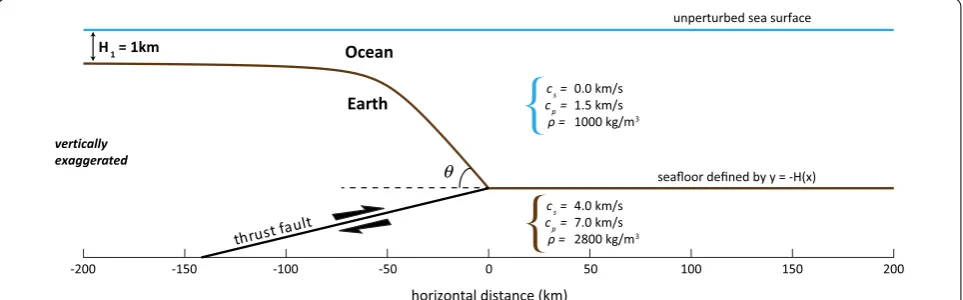
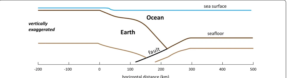
We employ two structural models in this study. The first is an idealized subduction zone geometry with a homogeneous solid Earth, and the second is based on our previous studies of the 2011 Tohoku earthquake (Koz-don and Dunham 2013, 2014). In the idealized model, an ocean with a sloping seafloor rests above a homoge-neous solid Earth, with a planar thrust fault intersecting the seafloor at its deepest point (Fig. 3). The fault dips at 10◦. This shallowly dipping fault is typical of subduc-tion zone plate boundaries, especially near the trench (e.g., Kopp and Kukowski 2003; Gutscher et al. 2001). The seafloor bathymetry to the right of the trench is flat, for simplicity. To the left of the trench, the bathymetry is set by a hyperbolic curve that asymptotes to horizontal away from the trench and to a slope of angle θ near the trench.
We vary θ across simulations, which changes the depth
of the trench and the slope of the seafloor. Results with different θ are all qualitatively similar, so only simulations
with θ =10◦ are reported here. The vertical position of the seafloor is defined as y= −H(x); y= −H1= −1 km
at the landward (left) side of the domain and y= −10 km
at the trench for θ =10◦. The trench is slightly deeper than in most subduction zones, but this hyperbolic sea-floor shape is a simple way to parameterize the geometry while avoiding too many free parameters.
Although real subduction zones often have compliant sedimentary prisms that affect the rupture process (Lotto et al. 2017), here we assume for simplicity in our idealized structural models that the Earth has homogeneous mate-rial properties, with s-wave speed cs=4.0 km/s, p-wave
-200 -150 -100 -50 0 50 100 150 200
horizontal distance (km) vertically
exaggerated
unperturbed sea surface
seafloor defined by y = -H(x) Earth
Ocean
thrust fault
H1 = 1km
θ
cs = cp =
ρ = 0.0 km/s 1.5 km/s 1000 kg/m3
cs = cp = ρ =
4.0 km/s 7.0 km/s 2800 kg/m3
speed cp=7.0 km/s, and density ρ=2800 kg/m3 . In the
ocean, cs=0, cp=1.5 km/s, and ρ=1000 kg/m3. The
gravitational acceleration is g=9.8 m/s2.
The full-physics model initiates with an earthquake on the fault. For the purposes of this study, either a kinematic or dynamic source model could be used. We choose to use a dynamic rupture model where slip is controlled by the interplay between elastodynamics and a fault friction law. For simulations using the idealized structural model, we nucleate rupture on the fault at the point x= −75 km , where x=0 defines the position of the trench. The rup-ture propagates along the entire ∼140-km length of the fault according to the rate-and-state friction law (Kozdon and Dunham 2013):
with the steady-state friction coefficient given by
where T is the shear strength of the fault, σ¯ is the effective
normal stress, V is the slip velocity, l=0.8 m is the state
evolution distance, f0=0.6 is the friction coefficient for
steady sliding at reference velocity V0=1µm/s, b=0.02 ,
and a=0.016. The dimensionless parameter b−a determines whether friction increases or decreases with changes to V. Since b−a=0.004 for our simulations,
friction is velocity-weakening and unstable slip can occur. In order to account for poroelastic changes in pore pressure, p, as a response to changes in total normal stress, �σ, we use the linear relation �p=B�σ, with B=0.6. The poroelastic effect alters effective normal
stress as Kozdon and Dunham (2013)
(10) dT
dt = aσ¯
V tanh T
aσ¯ dV
dt − V
l
|T| − ¯σfss(V),
(11)
fss(V)=f0−(b−a)ln(V/V0),
which serves to partially buffer the changes in effective normal stress. Equation (12) is a limiting case of a model (Cocco and Rice 2002) where the fault is surrounded by highly damaged material; in that limit, B is Skempton’s coefficient.
Initial effective normal stress σ¯0 is calculated as the
difference between normal stress in the Earth and pore pressure. Normal stress on the fault is set to lithostatic, and pore pressure is hydrostatic; effective normal stress increases with depth to a maximum of σ¯0=40 MPa, at
which point pore pressure increases lithostatically. Initial shear stress on the fault, T0, is set to T0=0.6σ¯0.
We compare the results of the full-physics model to those of a 2-D linearized shallow water wave model (i.e., Eqs. 1, 2), for which we use the same bathymetry as the full-physics model and set initial conditions based on the results of the full-physics model as follows. To set the initial sea surface height, η0(x), we first run a simulation
using the full-physics model where we set the gravita-tional acceleration to g =0 so that surface gravity waves do not propagate. After seismic and ocean acoustic waves propagate out of the domain, the sea surface is statically perturbed in a profile that resembles the seafloor dis-placement but with short wavelength variations filtered out (Kajiura 1963; Lotto and Dunham 2015; Saito 2013). This static sea surface perturbation becomes the initial condition on η0(x) for the shallow water model.
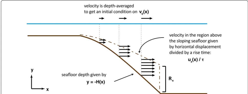
We set the initial condition on depth-averaged velocity v0(x) using the expressions provided by Song et al. (2008)
and are summarized in Eqs. (8) and (9) and Fig. 4. Here, ux(x) is taken from the final displacement of the seafloor (12)
¯
σ = ¯σ0+(1−B)�σ,
y = -H(x)
velocity in the region above the sloping seafloor given by horizontal displacement divided by a rise me:
seafloor depth given by
velocity is depth-averaged to get an initial condition on v0(x)
ux(x) / τ
x y
R
xin the zero gravity version of the full-physics simulation, Rx comes from the model geometry, and the rise time τ is
a free parameter that we vary to control the amplitude of the initial velocity.
Comparing full‑physics to shallow water simulations
Here, we compare the results of the shallow water model to those of the full-physics model, using the ide-alized material structure and geometry for both mod-els. In order to make a proper comparison, we must first account for a time delay that comes about because the full-physics model begins with an earthquake rupture that generates the tsunami over tens of seconds whereas the shallow water model is initialized at time t=0 with a tsunami profile already in place. We calculate the time delay by comparing η(x,t) at each time step of the full-physics simulation to the initial profile η0(x) of the
equivalent shallow water simulation (which, as described previously, is set by a zero gravity full-physics simula-tion). We calculate the misfit with respect to η0(x) at each
time step using the L2 norm, with the time of minimum
misfit is taken to be the time delay between the full-phys-ics model and the shallow water model. Alternatively, we can calculate the time delay by selecting some time step of η(x,t) in the full-physics model after which all acous-tic waves have exited the domain and matching η(x,t) of the shallow water model, subject to some time delay, to that in the full-physics model. The time delay from this alternate approach yields basically the same results as the approach previously described. Though the time delay changes slightly between simulations, the offset is typi-cally ∼85 s, meaning that it takes about 85 s (roughly, the rupture duration) for the full-physics model to generate a tsunami profile that matches the initial condition of the shallow water code.
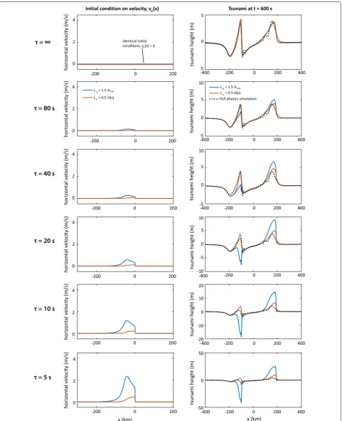
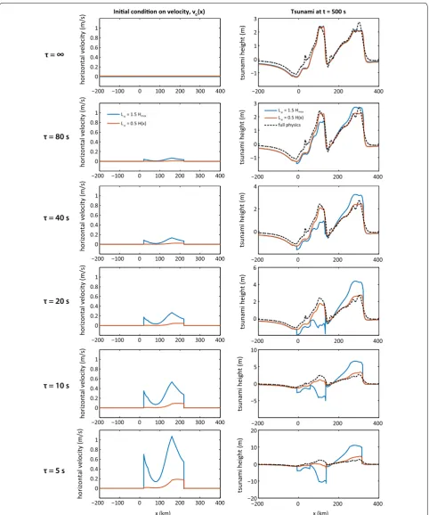
We run two sets of shallow water simulations with initial horizontal velocity set by Eqs. (8) and (9), one using LH =1.5Hmax and the other using LH =0.5H(x) .
The only remaining free parameter is the rise time τ,
for which Song et al. use a value of τ ∼5–20 s for their Sumatra and Tohoku simulations (Song and Han 2011; Xu and Song 2013; Song et al. 2017). We vary τ over a
much larger range, as we find that using τ ∼5–20 s leads to tsunami waves of unrealistically large amplitudes, as evident in the bottom rows of Fig. 5.
Rather, we find that the shallow water tsunami best fits the full-physics tsunami when rise time τ approaches
infinity (top rows of Fig. 5), i.e., when v0(x)=0. Note that
even when tsunami amplitudes match, the waveforms do not align perfectly because the tsunami experiences dis-persion of short wavelengths in the full-physics model but not in the shallow water model. With τ interpreted
as the local rise time, setting τ = ∞ is inconsistent with
the assumption that the seafloor completes its deforma-tion over a timescale smaller than the tsunami propaga-tion time over horizontal wavelengths characterizing the deformation profile. However, more generally τ can
be viewed simply as a scalar parameter that controls the amplitude of the initial velocity, with the shape or profile still given by Eqs. (8) and (9).
Shallow water models with non-negligible initial veloc-ity (i.e., those with finite rise times) produce the same sort of asymmetry in tsunami waveform as illustrated in the simple example in Fig. 2. In contrast, the full-physics simulation yields a tsunami profile that is nearly symmet-rical in amplitude between seaward and landward waves, though this is complicated somewhat by the nonuniform ocean depth.
We can quantify the misfit between the tsunamis pro-duced by the shallow water and full-physics models by taking the 2 norm of the difference between the final sea surface heights plotted in Fig. 5. Those misfits are shown in Fig. 8a. The misfit is never zero because the full-phys-ics model accounts for the finite source duration, sur-face gravity wave dispersion, and ocean compressibility, which are neglected in the shallow water model. For either choice of LH, the smallest misfits occur in the limit
as rise time approaches infinity, i.e., τ → ∞ so v0→0 .
When using LH =0.5H(x), we find that misfits are nearly
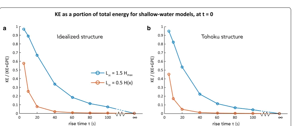
at their minimum for τ ≥40 s. In Fig. 9a, we plot kinetic
energy (KE) as a portion of the total energy in the ocean at the initial time step of each shallow water simula-tion. We define energy and discuss it more thoroughly in “Energy considerations” section, but for now it is suffi-cient to view KE as a quantitative scalar measure of parti-cle velocities in the ocean. By comparison with Fig. 8a, we observe that models with minimum misfit are the same as those with negligible initial KE. In other words, even though models with LH =0.5H(x) and τ ≥40 s produce
small misfits, they only do so because they essentially have zero initial horizontal velocities.
Tohoku simulations
horizontal velocity (m/s
)
LH = 1.5 Hmax LH = 0.5 H(x)
-200 0 200
0 2 4
-400 -200 0 200 400
-5 0 5
tsunami height (m
)
LH = 1.5 Hmax LH = 0.5 H(x) full physics simulation
horizontal velocity (m/s
)
-200 0 200
0 2 4
-400 -200 0 200 400
-5 0 5 10
tsunami height (m
)
horizontal velocity (m/s
)
-200 0 200
0 2 4
-400 -200 0 200 400 -5
0 5 10
tsunami height (m
)
horizontal velocity (m/s
)
-200 0 200
0 2 4
-400 -200 0 200 400
-10 -5 0 5 10
tsunami height (m
)
horizontal velocity (m/s
)
0
-200 0 200
0 2 4
-400 -200 0 200 400 -20
-10 10 20
tsunami height (m
)
x (km)
horizontal velocity (m/s
)
x (km)
-200 0 200
0 2 4
-400 -200 0 200 400 -50
0 50
tsunami height (m
)
τ = ∞
τ = 80 s
τ = 40 s
τ = 20 s
τ = 10 s
τ = 5 s
Initial condition on velocity, v0(x) Tsunami at t = 600 s
identical initial condions, v0(x) = 0
Fig. 5 Comparisons of shallow water wave simulations with full-physics simulations for θ=10◦, where each row uses a different value of rise time τ
Note that, as seen in Fig. 6, the ocean layer rises above and covers the land in an unphysical way. This is an arti-fact of the way we break our full-physics model into cur-vilinear computational “blocks,” but it does not affect our results as long as we are interested in tsunami propaga-tion prior to wave arrival at the coast.
Just as we did for the simplified geometry in the pre-vious section, we run two shallow water simulations set-ting initial horizontal velocity with Eqs. (8) and (9), one using LH =1.5Hmax and the other using LH =0.5H(x).
The bathymetry of the full-physics simulation determines H(x) in the shallow water models, and the initial condi-tion η0(x) comes from the final displacement of the sea
surface in a full-physics Tohoku simulation with no grav-ity. As with the idealized geometry simulations, the time delay between the full-physics and shallow water simula-tions is calculated by finding the time step of least misfit between η(x,t) of the full-physics model and η0(t) of the
shallow water model. For the Tohoku geometry, that mis-fit is ∼70 s.
The results, shown in Fig. 7, demonstrate once again that the best choice for rise time using the Song et al. approach in Eq. (8) is τ = ∞, i.e., v0(x)=0. We quantify
the misfits between the final tsunamis produced by the shallow water and full-physics models in Fig. 8b, and we observe that misfits are lowest as τ → ∞ and v0→0 .
Just as in the previous section, misfits are at their mini-mum when initial kinetic energy (KE) in the ocean is neg-ligible (Fig. 9b), i.e., when v0(x)=0. These results do not
indicate that v0(x)=0 is the correct, or even most
self-consistent, choice for an initial condition on horizontal velocity for shallow water models, as this experiment explores only two possible initial velocity profiles. How-ever, the results do imply that with these velocity profiles, the Song et al. theory makes inconsistent predictions of the tsunami, especially when choosing τ =5−20 s.
We furthermore see no evidence arguing against using
v0(x)=0 as the initial velocity for most tsunami
mod-eling problems.
Adjoint problem
Next, we use an alternative approach to determine tsu-nami initial conditions that avoids any assumptions regarding the initial velocity profile. In concept, the opti-mal way to constrain the initial condition on horizontal velocity is through direct examination of the particle velocity field of our full-physics model. If we integrate horizontal velocity over the ocean depth at an appropri-ate “initial” time, we could simply use that horizontally variable, depth-averaged velocity profile as an initial condition for a shallow water simulation. However, this approach is unfeasible: Setting aside the question of how to select an initial time, our full-physics model produces large amplitude seismic and ocean acoustic waves that interfere with the wavefield of the tsunami for the first few hundred seconds. This makes it impossible to iso-late the tsunami particle velocity from the total particle velocity for use in setting the initial condition on v0(x).
However, appropriate (i.e., self-consistent) tsunami initial conditions can be determined using the following adjoint wavefield procedure. We first run a full-physics simulation (with the same idealized structure as in Fig. 3) for 1000 s of simulation time, long enough for all seismic and acoustic waves to exit through the boundaries of the domain, leaving only the slower-propagating tsunami in the ocean. Having isolated the tsunami, we then use the stress and velocity fields at the end of this first simula-tion as an initial condisimula-tion on a time-reversed adjoint simulation. In addition to running backward in time, the adjoint simulation involves flipping the sign of the particle velocity. Since the wave propagation problem is self-adjoint, no changes are required to the code to per-form an adjoint simulation. In the adjoint simulation, the tsunami propagates backward in time, and landward and horizontal distance (km)
sea surface
seafloor
vertically exaggerated
fault
Earth
Ocean
-200 -100 0 100 200 300 400 500
−200 −100 0 100 200 300 400
Inial condion on velocity, v0(x) Tsunami at t = 500 s
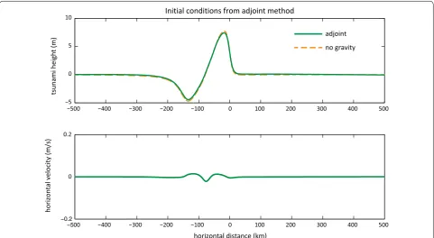
seaward propagating tsunami waves converge above the earthquake source into the initial tsunami profile. We determine the initial condition by finding the time where the sea surface profile from the adjoint simulation best matches the sea surface profile of the equivalent forward simulation with zero gravity (as in the top of Fig. 10). The sea surface height and depth-averaged horizontal veloc-ity fields at this time are identified as η0(x) and v0(x), the
initial conditions that are most consistent with the full-physics simulations.
Not surprisingly, we can find a time step in the adjoint problem where the tsunami profile very closely matches that of the equivalent zero gravity simulation. At this time step, the depth-averaged horizontal velocity in the ocean is of order 10−2 m/s and appears in a profile that does not
match either of those profiles suggested by Song et al.
rise time τ (s) 101
102 103
misfi
t
LH = 1.5 Hmax
LH = 0.5 H(x)
0 20 40 60 80 100 ∞ 10
1
102 103
misfi
t
rise time τ (s)
0 20 40 60 80 100 ∞
Misfits for idealized structure Misfits for Tohoku structure
a b
Fig. 8 Misfit between the sea surface height of full-physics simulations and shallow water simulations, calculated at the final time step plotted in previous figures using the L2 norm. a Misfits for the idealized structure in Fig. 3, calculated at t=600 s as in Fig. 5. b Misfits for the Tohoku geometry in Fig. 6, calculated at t=500 s as in Fig. 7. For both sets of simulations and both choices of LH, misfit is minimized as rise time τ approaches infinity (initial velocity v0→0)
0 0.1 0.2 0.3 0.4 0.5 0.6 0.7 0.8 0.9 1
rise time τ (s)
0 20 40 60 80 100 ∞
KE / (KE+GPE
)
KE as a portion of total energy for shallow-water models, at t = 0
0 0.1 0.2 0.3 0.4 0.5 0.6 0.7 0.8 0.9 1
KE / (KE+GPE
)
rise time τ (s)
0 20 40 60 80 100 ∞
a b
LH = 1.5 Hmax LH = 0.5 H(x)
Idealized structure Tohoku structure
The adjoint calculation suggests that the self-consistent initial condition is one that has nonzero, but very small, horizontal velocity. This result does not corroborate the shape of either of the profiles proposed by Song et al., nor is the velocity amplitude consistent with predicted initial velocity using the rise times that Song et al. recommend.
Energy considerations
Song et al. (2008, 2017), Song and Han (2011), and Titov et al. (2016) have frequently brought the concept of energy into their discussion of tsunamis, making esti-mates of kinetic energy (KE) and gravitational potential energy (GPE) in the ocean, immediately after the earth-quake prior to tsunami propagation, and attributing the kinetic energy to momentum transfer from the horizon-tal motion of the seafloor during tsunami generation. In this section, we calculate the energy balance of the ocean for the full-physics model using the idealized geometry discussed in a previous section.
In addition to KE and GPE, in our full-physics frame-work we must additionally consider the stored compres-sional energy in the ocean, which we refer to as acoustic energy (AE) (Lotto and Dunham 2015). More precisely, the AE is the recoverable internal energy associated with com-pressing or expanding the water. We define the total energy in the ocean, E, as the sum of these three components:
where v is the total velocity, p is the pressure, K =ρc2 p
is the bulk modulus of water, and D=5000 km is the
horizontal distance from the trench to either end of the domain. Energy can escape out of the side boundaries as waves pass through the edges of the domain.
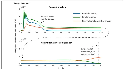
Figure 11 tracks the components of E over time for the same full-physics simulation discussed in “Adjoint prob-lem” section. An earthquake nucleates at time t=0, gen-erating seismic waves and deforming the elastic solid. The solid Earth does work on the ocean through normal trac-tions on the seafloor, transferring energy into the ocean in the form of acoustic waves and surface gravity waves. The fast-moving acoustic waves propagate out of the domain within the first few hundreds of seconds of simu-lation time, carrying with them much of the KE and AE. After about 300 s, only the tsunami remains within the (13)
E =KE+AE+GPE
=
0
−H(x)
D
−D 1
2ρ
v2dxdy
+
0
−H(x)
D
−D 1
2Kp 2
dxdy
+
D
−D 1 2ρgη
2
dx,
−500 −400 −300 −200 −100 0 100 200 300 400 500
−5 0 5
10 Initial conditions from adjoint method
tsunami height (m
)
−0.2
0 0.2
horizontal velocity (m/s
)
horizontal distance (km)
adjoint no gravity
−500 −400 −300 −200 −100 0 100 200 300 400 500
domain, with relatively constant KE and GPE of approxi-mately equal amplitudes and negligible AE.
At t=1000 s, we begin to run the adjoint problem with
reversed time. In the adjoint problem, there is no source of acoustic waves and so the AE continues to be negligi-ble. Both GPE and KE remain relatively constant until the tsunamis that were propagating in opposite directions begin to interfere with each other in the source region. This interference establishes the tsunami initial conditions, with the dashed line in Fig. 11 corresponding to the initial conditions shown in Fig. 10. At this time, virtually all of the energy in the ocean is GPE, with negligible KE, such that KE/(KE + GPE) = 0.002. This observation argues against the claim of Song et al. that the KE of the initial tsunami is higher (or even significantly higher) than the GPE.
However, it is important to note that our energy bal-ance calculation provides quantitative support for the impulse-momentum theory promoted by Song et al. There is indeed a considerable amount of KE imparted to the ocean by the solid Earth during the tsunami gen-eration process. However, almost all of this KE is cou-pled with AE in the form of acoustic waves, rather than remaining in the vicinity of the tsunami source region to provide a non-negligible contribution to initial velocity.
Discussion and conclusions
We have taken two unique approaches in our attempt to determine the appropriate initial condition on horizontal velocity v0(x) for shallow water tsunami models. The first
approach involves running comparable tsunami simula-tions with a full-physics model and a linearized shallow water wave model, and selecting the initial condition on horizontal velocity for the shallow water model using the expressions presented by Xu and Song (2013), Titov et al. (2016) and Song et al. (2017). We then vary the rise time parameter τ, which scales the amplitude of v0(x), and
compare the tsunamis predicted by the shallow water and full-physics simulations.
This comparison is made for two model geometries: an idealized subduction zone geometry (Fig. 3) and a 2011 Tohoku earthquake geometry (Fig. 6). For both geom-etries, our simulations unequivocally demonstrate that the initial condition on v0(x) (Eqs. 8, 9) using τ = 5–20
s, as Song et al. have suggested, overestimates tsunami amplitudes by several times. Tsunami amplitudes are nearly an order of magnitude too large when choosing LH =1.5Hmax, as Song et al. have done in more than one
publication (Song and Han 2011; Xu and Song 2013). If we use larger values for τ – which may be more physically
0 100 200 300 400 500 600 700 800 900 1000
0 2 4 6 x 10
10
time (s)
energy per unit horizontal distance (J/m
)
Energy in ocean
1000 900 800 700 600 500 400 300 200 100 0
0 2 4 6 x 10
10
Acoustic energy Kinetic energy
Gravitational potential energy
Forward problem
Adjoint (time-reversed) problem
Acoustic waves exit the domain
time of initial conditions from adjoint method
relevant because the rupture process for typical tsu-namigenic earthquakes lasts several tens of seconds— we find that the shallow water model produces results closer to the full-physics simulations, especially when
LH =0.5H(x). But when τ ≥80 s and LH =0.5H(x), the
initial horizontal velocity profile is nearly flat, virtually indistinguishable from choosing v0(x)=0, i.e., τ = ∞.
Quantitative measures of misfit between the two models (Fig. 8) support the conclusion that shallow water simu-lations best match their full-physics counterparts as rise time τ approaches infinity. Indeed, comparing Figs. 8 and 9 reveals that any shallow water simulation that reason-ably matches its full-physics counterpart does so because initial KE—and, accordingly, initial horizontal velocity— is negligible.
The second approach requires us to run a full-phys-ics simulation long enough for all seismic and acoustic waves to leave the domain, and then to run it backward in time to solve the adjoint problem. This adjoint simula-tion method allows us to use the full-physics simulasimula-tion to directly determine v0(x). In doing so, we again find
that v0(x) is so small in magnitude so as to be practically
equivalent to the null hypothesis, v0(x)=0. This method
produces a velocity profile that does not qualitatively match that suggested by Song et al. Most notably, the initial velocity profile determined by the adjoint method does not reach its maximum at the trench (x=0 ) and is not uniformly positive. We also find that at the time of this adjoint-based initial condition, almost all the energy in the ocean is in the form of gravitational potential energy and virtually none is kinetic energy.
We conclude that Song et al.’s proposed choice of v0(x)
for modeling tsunamis will consistently overestimate tsu-nami heights. Furthermore, we have found no convincing evidence of any better choice than v0(x)=0, which is the
default initial condition on horizontal velocity used by most tsunami modelers.
In a study published after initial submission of our manuscript, Song et al. tested their tsunami generation theory by comparing simulations using initial condition (8 and 9) to tide gauge and DART data from the 2011 Tohoku event (Song et al. 2017). They argued that their tsunami generation theory matches the data better than the conventional tsunami generation theory. However, many other authors have successfully used the standard initial condition v0(x)=0 to fit data both landward and
seaward of the rupture area (Bletery et al. 2014; Gusman et al. 2012; Hooper et al. 2013; Satake et al. 2013). The fits are equally good. This suggests that there is sufficient nonuniqueness with regard to the tsunami initial condi-tions given the available tsunami data from the Tohoku event. It follows that we cannot equivocally disambiguate
between Song’s initial conditions and the conventional initial conditions from even this well-recorded tsunami.
Song et al. have also used laboratory wave basin tests to create an empirical scaling relationship between the ratio of initial kinetic to gravitational potential energy (KE/GPE) and a normalized version of tsunami amplitude (Song et al.
2017). Using characteristic values for ocean depth, fault slip, rise time, and tsunami amplitude, they fit the 2011 Tohoku and 2004 Sumatra tsunamis into this paradigm. A full discussion of these laboratory experiments is beyond the scope of this paper, but we note certain flaws in the scal-ing relations of the experiments. First, tsunami amplitudes in the open ocean are much smaller than ocean depths (|η|/H ≪1), but in these experiments |η|/H≈0.1−0.7. Nonlinearity is therefore essential in the experiments, while negligible in the real ocean. Second, water compressibility effects are vastly less important in the experiments than in the real ocean. Two dimensionless parameters quantify-ing compressibility effects are gH/c2 and H/cτ, where c is the sound speed in the ocean and τ is again the rise time
or source duration. These dimensionless parameters, and therefore compressibility effects, are several orders of mag-nitude more important in real tsunamis than in the experi-ments. These differences in scaling suggest that waves in these laboratory experiments are generated and propagate in a different manner from real tsunamis.
What accounts for the stark difference between the results in this paper and in the studies of Song and col-laborators? In our full-physics simulations, we observe large amplitude acoustic waves in the ocean, likely due in part to the transfer of horizontal momentum from the solid Earth to the ocean during earthquake rupture. Our full-physics model, which includes a compressible ocean, captures these acoustic waves that a model using an incompressible ocean would miss. In an incompress-ible ocean with a finite domain, horizontal momentum transferred from the solid Earth to the ocean would be left in the vicinity of the source region rather than being carried away by acoustic waves. However, in a full-phys-ics, compressible ocean model most of the kinetic energy injected into the ocean by the seafloor displacement is carried away by acoustic waves and does not significantly contribute to tsunami height. Overall, we conclude that the standard practice of setting initial horizontal velocity to zero remains the best, and most consistent, procedure for tsunami modeling.
Authors’ contributions
Author details
1 Department of Geophysics, Stanford University, Stanford, CA, USA. 2 Institute
for Computational and Mathematical Engineering, Stanford University, Stan-ford, CA, USA. 3 Department of Electrical Engineering and Computer Sciences,
University of California – Berkeley, Berkeley, CA, USA.
Acknowlegements
We thank the two anonymous reviewers for constructive comments and Tatsuhiko Saito for insightful discussions regarding tsunami generation.
Competing interests
The authors declare that they have no competing interests.
Availability of data and materials
All modeling results, along with MATLAB scripts to read them, will be shared freely upon request.
Consent for publication Not applicable.
Ethics approval and consent to participate Not applicable.
Funding
This work was supported by the National Science Foundation (EAR-1255439).
Publisher’s Note
Springer Nature remains neutral with regard to jurisdictional claims in pub-lished maps and institutional affiliations.
Received: 18 May 2017 Accepted: 8 August 2017
References
Behrens J, Androsov A, Babeyko AY, Harig S, Klaschka F, Mentrup L (2010) A new multi-sensor approach to simulation assisted tsunami early warning. Nat Hazards Earth Syst Sci 10(6):1085–1100
Bernard EN, Mofjeld HO, Titov V, Synolakis CE, González FI (2006) Tsunami: scientific frontiers, mitigation, forecasting and policy implications. Philos Trans R Soc Lond A Math Phys Eng Sci 364(1845):1989–2007
Bletery Q, Sladen A, Delouis B, Vallée M, Nocquet J-M, Rolland L, Jiang J (2014) A detailed source model for the Mw9. 0 Tohoku-Oki earthquake reconcil-ing geodesy, seismology, and tsunami records. J Geophys Res Solid Earth 119(10):7636–7653
Borrero JC, Sieh K, Chlieh M, Synolakis CE (2006) Tsunami inundation modeling for western Sumatra. Proc Natl Acad Sci 103(52):19673–19677
Cocco, M, Rice, JR (2002) Pore pressure and poroelasticity effects in Coulomb stress analysis of earthquake interactions. J Geophys Res Solid Earth 107(B2):ESE 2-1–ESE 2-17
Fujii Y, Satake K, Sakai S, Shinohara M, Kanazawa T (2011) Tsunami source of the 2011 off the Pacific coast of Tohoku Earthquake. Earth Planets Space 63(7):55. doi:10.5047/eps.2011.06.010
Geist EL, Parsons T (2006) Probabilistic analysis of tsunami hazards. Nat Hazards 37(3):277–314
González FI, Geist EL, Jaffe B, Kânoğlu U, Mofjeld H, Synolakis CE, Titov VV, Arcas D, Bellomo D, Carlton D, et al (2009) Probabilistic tsunami hazard assess-ment at Seaside, Oregon, for near-and far-field seismic sources. J Geophys Res Oceans 114:C11023
Gusman AR, Tanioka Y, Sakai S, Tsushima H (2012) Source model of the great 2011 Tohoku earthquake estimated from tsunami waveforms and crustal deformation data. Earth Planet Sci Lett 341:234–242
Gutscher M-A, Klaeschen D, Flueh E, Malavieille J (2001) Non-coulomb wedges, wrong-way thrusting, and natural hazards in Cascadia. Geology 29(5):379–382
Hooper A, Pietrzak J, Simons W, Cui H, Riva R, Naeije M, Terwisscha A, van Scheltinga E, Schrama G Stelling, Socquet A (2013) Importance of horizontal seafloor motion on tsunami height for the 2011 Mw = 9.0 Tohoku-Oki earthquake. Earth Planet Sci Lett 361:469–479
Kajiura K (1963) The leading wave of a tsunami. Bull Earthq Res Inst 43:535–571 Kajiura K (1970) Tsunami source, energy and the directivity of wave radiation.
Bull Earthq Res Inst Univ Tokyo 48:835–869
Kopp H, Kukowski N (2003) Backstop geometry and accretionary mechanics of the Sunda margin. Tectonics 22(6):1072
Kowalik Z (2003) Basic relations between tsunamis calculation and their physics-ii. Sci Tsunami Hazards 21(3):154–173
Kozdon JE, Dunham EM (2013) Rupture to the trench: dynamic rupture simula-tions of the 11 March 2011 Tohoku earthquake. Bull Seismolog Soc Am 103(2B):1275–1289
Kozdon JE, Dunham EM (2014) Constraining shallow slip and tsunami excita-tion in megathrust ruptures using seismic and ocean acoustic waves recorded on ocean-bottom sensor networks. Earth Planet Sci Lett 396:56–65
Lotto GC, Dunham EM (2015) High-order finite difference modeling of tsunami generation in a compressible ocean from offshore earthquakes. Comput Geosci 19:327–340
Lotto GC, Dunham EM, Jeppson TN, Tobin HJ (2017) The effect of compliant prisms on subduction zone earthquakes and tsunamis. Earth Planet Sci Lett 458:213–222
Maeda T, Furumura T (2013) FDM simulation of seismic waves, ocean acoustic waves, and tsunamis based on tsunami-coupled equations of motion. Pure Appl Geophys 170(1–2):109–127
Melgar D, Bock Y (2013) Near-field tsunami models with rapid earthquake source inversions from land-and ocean-based observations: the potential for forecast and warning. J Geophys Res Solid Earth 118(11):5939–5955 Mori N, Takahashi T, Yasuda T, Yanagisawa H (2011) Survey of 2011 Tohoku
earthquake tsunami inundation and run-up. Geophys Res Lett 38(7):L00G14
Saito T (2013) Dynamic tsunami generation due to sea-bottom deformation: analytical representation based on linear potential theory. Earth Planets Space 65(12):1411–1423. doi:10.5047/eps.2013.07.004
Saito T, Furumura T (2009) Three-dimensional tsunami generation simulation due to sea-bottom deformation and its interpretation based on the linear theory. Geophys J Int 178(2):877–888
Satake K (2002) Tsunamis. Int Geophys 81:437–451
Satake K, Fujii Y, Harada T, Namegaya Y (2013) Time and space distribution of coseismic slip of the 2011 Tohoku earthquake as inferred from tsunami waveform data. Bull Seismol Soc Am 103(2B):1473–1492
Sato M, Ishikawa T, Ujihara N, Yoshida S, Fujita M, Mochizuki M, Asada A (2011) Displacement above the hypocenter of the 2011 Tohoku-Oki earthquake. Science 332(6036):1395–1395
Song YT, Fu L-L, Zlotnicki V, Ji C, Hjorleifsdottir V, Shum CK, Yi Y (2008) The role of horizontal impulses of the faulting continental slope in generating the 26 December 2004 tsunami. Ocean Model 20(4):362–379
Song YT, Han S-C (2011) Satellite observations defying the long-held tsunami genesis theory. In: Tang DL (ed) Remote sensing of the changing Oceans, Springer, pp 327–342
Song YT, Mohtat A, Yim SC (2017) New insights on tsunami genesis and energy source. J Geophys Res Oceans 122(5):4238–4256
Tanioka Y, Satake K (1996) Tsunami generation by horizontal displacement of ocean bottom. Geophys Res Lett 23(8):861–864
Titov V, Song YT, Tang L, Bernard EN, Bar-Sever Y, Wei Y (2016) Consistent esti-mates of tsunami energy show promise for improved early warning. Pure Appl Geophys 173(12):3863–3880
Titov VV, Gonzalez FI (1997) Implementation and testing of the method of splitting tsunami (MOST) model. Technical Report NOAA Tech. Memo. ERL PMEL-112 (PB98-122773), NOAA/Pacific Marine Environmental Laboratory, Seattle, WA
Titov VV, Gonzalez FI, Bernard EN, Eble MC, Mofjeld HO, Newman JC, Venturato AJ (2005) Real-time tsunami forecasting: challenges and solutions. In: Bernard EN (ed) Developing tsunami-resilient communities, Springer, pp 41–58
Titov VV, Synolakis CE (1998) Numerical modeling of tidal wave runup. J Waterw Port Coast Ocean Eng 124(4):157–171
Watts P, Grilli ST, Kirby JT, Fryer GJ, Tappin DR (2003) Landslide tsunami case studies using a Boussinesq model and a fully nonlinear tsunami genera-tion model. Nat Hazards Earth Syst Sci 3(5):391–402