Evaluation of String Distance Algorithms for Dialectology
Wilbert Heeringa, Peter Kleiweg, Charlotte Gooskens & John Nerbonne Humanities Computing, University of Groningen
{W.J.Heeringa, P.C.J.Kleiweg, C.S.Gooskens, J.Nerbonne}@rug.nl
Abstract
We examine various string distance mea-sures for suitability in modeling dialect distance, especially its perception. We find measures superior which do not normalize for word length, but which are are sensi-tive to order. We likewise find evidence for the superiority of measures which incor-porate a sensitivity to phonological con-text, realized in the form of n-grams— although we cannot identify which form of context (bigram, trigram, etc.) is best. However, we find no clear benefit in us-ing gradual as opposed to binary segmen-tal difference when calculating sequence distances.
1 Introduction
We compare string distance measures for their value in modeling dialect distances. Traditional dialectology relies on identifying language fea-tures which are common to one dialect area while distinguishing it from others. It has difficulty in dealing with partial matches of linguistic fea-tures and with non-overlapping language patterns. Therefore Seguy (1973) and Goebl (1982; 1984) advocate using aggregates of linguistic features to analyze dialectal patterns, effectively introducing the perspective ofDIALECTOMETRY.
Kessler (1995) introduced the use of string edit distance measure as a means of calculating the dis-tance between the pronunciations of correspond-ing words in different dialects. Followcorrespond-ing Seguy’s and Goebl’s lead, he calculated this distance for pairs of pronunciations of many words in many Irish-speaking towns. String edit distance is sen-sitive to the degrees of overlap of strings and
al-lows one to process large amounts of pronunci-ation data, including that which does not follow other isoglosses neatly. Heeringa (2004) exam-ines several variants of edit distance applied to Norwegian and Dutch data, focusing on measures which involve a length normalization, and which ignore phonological context, and demonstrating that measures using binary segment differences are no worse than those using feature-based mea-sures of segment difference.
This paper inspects a range of further refine-ments in measuring pronunciation differences. First, we inspect the role of normalization by length, showing that it actually worsens non-normalized measures. Second, we compare edit distance measures to simpler measures which ig-nore linear order, and show that order-sensitivity is important. Third, we inspect measures which are sensitive to phonetic context, and show that these, too, tend to be superior. Fourth, we com-pare versions of string edit distance which are constrained to respect syllable structure (always matching vowels with vowels, etc.), and conclude that this is mildly advantageous. Finally we com-pare binary (i.e., same/different) treatments of the segments in edit distance to gradual treatments of segment differentiation, and find no indication of the superiority of the gradual measures.
The quality of the measures is assayed primarily through their agreement with the judgments of di-alect speakers about which varieties are perceived as more similar (or dissimilar) to their own. In addition we inspect a validation technique which purports to show how successfully a dialect mea-sure uncovers the geographic structure in the data (Nerbonne and Kleiweg, 2006), but this technique yields unstable results when applied to our data. We have perception data only for Norwegian, so
that data figures prominently in our argument, and we evaluate both Norwegian and German data ge-ographically.
The results differ, and the perceptual results (concerning Norwegian) are most easily inter-pretable. There we find, as noted above, that non-normalized measures are superior to normal-ized ones, that both order and context sensitiv-ity are worthwhile, as is the vowel/consonant dis-tinction. The (geographic) results for German are more complicated, but also less stable. We include them for the sake of completeness.
In addition we note two minor contributions. First, although some literature ends up evaluat-ing both distance and similarity measures, because these are not consistently each others’ inverses un-der some normalizations (Kondrak, 2005; Inkpen et al., 2005), we suggest a normalization based on alignment length which guarantees that similarity is exactly the inverse of distance, allowing us to concentrate on distance.
Second, we note that there is no great problem in applying edit distance to bigrams and trigrams, even though recent literature has been sceptical about the feasibility of this step. For example Kessler (2005) writes:
[...] one major shortcoming [in applying edit distance to linguistic data, WH et al] that is rarely discussed is that the pho-netic environment of the sounds in ques-tion cannot be taken into account, while still making use of the efficient dynamic programming algorithm (p. 253).
Somewhat further Kessler writes: “Currently, the predominant solution to this problem is to ignore context entirely.” In fact Kondrak (2005) applies edit distance straightforwardly using n-gram as basic elements. Our findings accord with Kon-drak’s, who also found no problem in applying edit distance usingn-grams, but we evaluate the tech-nique in its application to dialectology.
1.1 Background
Heeringa (2004) demonstrates that edit distance applied to comparable words (see below for ex-amples) is a superior measure of dialect distance when compared to unigram corpus frequency and also that it is superior to both the frequency of pho-netic features in corpora (a technique which Hop-penbrouwers & HopHop-penbrouwers (2001) had ad-vocated) and to the frequency of phonetic features
taken one word at a time. Heeringa compares these techniques using the results of a perception ex-periment we also employ below. Heeringa shows that word-based techniques are superior to corpus-based techniques, and moreover, that most word-based techniques perform about the same. We therefore ignore measures which view corpora as undifferentiated collections below and study only word-based techniques.
A further question was whether to compare words based on a binary difference between seg-ments or whether to use instead phonetic fea-tures to derive a more sensitive measure of seg-ment distance. It turned out that measures us-ing binary segment distinctions outperform the feature-based methods (see Heeringa, pp. 184– 186), even though a number of feature systems and comparisons of feature vectors were experimented with. We likewise accept these results (at least for present purposes) and focus exclusively on mea-sures using the binary segment distinctions below. Kondrak (2005) and Inkpen et al. (2005) present several methods for measuring string similarity and distance which complement Heeringa’s results nicely. We should note, however, that these pa-pers focus on other areas of application, viz., the problems of identifying (i) technical names which might be confused, (ii) linguistic cognates (words from the same root), and (iii) translational cog-nates (words which may be used as translational equivalences). Inkpen et al. consider 12 different orthographic similarity measures, including some in which the order of segments does not play a role (e.g., DICE), and others which use order in align-ment (e.g. edit distance). They further consider comparison on the basis of unigrams, bigrams, tri-grams and “xbitri-grams,” which are tritri-grams without the middle element. Some methods are similarity measures, others are distance measures. We return to this in Section 2.
1.2 This paper
com-paring the algorithmic results to the distances as perceived by the dialect speakers themselves. We likewise aimed to evaluate by calculating the de-gree to which a measure uncovers geographic co-hesion in dialect data, but as we shall see, this means of validation yields rather unstable results. In Section 5 we present results for the different methods and finally, in Section 6, we draw some conclusions.
2 String Comparison Algorithms
In this section we describe a number of string comparison algorithms largely following Inkpen et al. (2005). The methods can be classified ac-cording to different factors: representation (un-igram, b(un-igram, tr(un-igram, xbigram), comparison of n-grams (binary or gradual), status of order (with or without alignment), and type of align-ment (free or forced alignalign-ment with respect to the vowel/consonant distinction). We illustrate the methods with examples, in which we compare German and Dutch dialect pronunciations of the word milk.1
2.1 Contextual sensitivity
In the German dialect of Reelkirchen milk is pro-nounced as [mElk@]. The bigram notation is [–m mE El lk k@ @–] and the trigram notation is [––m –mEmElElk lk@k@–@––]. The same word is pro-nounced as [mEl@c¸] in the German dialect of Tann. The bigram and trigram representations are [–m mE El l@ @c¸ c¸–] and [––m –mEmElEl@l@c¸@c¸– c¸––] respectively.
In the simplest method we present in this paper, the distance is found by calculating 1 minus twice the number of shared segmentn-grams divided by the total number ofn-grams in both words. Inkpen et al. mention a bigram-based, a trigram-based and a xbigram-based procedure, which they call DICE, TRIGRAM and XDICE respectively. We also consider an unigram-based procedure which we call UNIGRAM. The two pronunciations share four unigrams: [m,E, l] and [@]. There are5 + 5 = 10unigram tokens in total in the two words, so the unigram similarity is (2×4)/10 = 0.8, and the distance1−0.8 = 0.2. The two pronunciations share three bigrams: [–m, mE] and [El]. There are 6 + 6 = 12 bigram tokens in the two strings, so bigram similarity is(2×3)/12 = 0.5, and the dis-tance1−0.5 = 0.5. Finally, the two
pronuncia-1Our transcriptions omit diacritics for simplicity’s sake.
tions have three trigrams in common: [––m, –mE] and [mEl] among7+7 = 14in total, yielding a tri-gram similarity of(2×3)/14 = 0.4and distance 1−0.4 = 0.6.
Our interest in this issue is linguistic: longer
n-grams allow comparison on the basis of phonic context, and unigram comparisons have correctly been criticized for ignoring this (Kessler, 2005).
2.2 Order of segments
When comparing the German dialect pronuncia-tion of Reelkirchen [mElk@] with the Dutch dialect pronunciation of Haarlem [mEl@k], the unigram procedure presented above will detect no differ-ence. One might argue that we are dealing with a swap, but this is effectively an appeal to order. The example is not convincing for n-gram mea-sures, n ≥ 2, but we should prefer to separate issues of order from issues of context sensitivity. We use edit distance (aka Levenshtein distance) for this purpose, and we assume familiarity with this (Kruskal, 1999). In our use of edit distance all operations have a cost of 1.
2.3 Normalization by length
When the edit distance is divided by the length of the longer string, Inkpen et al. call it normal-ized edit distance (NED). In our approach we di-vide “raw edit distance” by alignment length. The same minimum distance found by the edit distance algorithm may be obtained on the basis of sev-eral alignments which may have different lengths. We found that the longest alignment has the great-est number of matches. Therefore we normalize by dividing the edit distance by the length of the longest alignment.
We have normally employed a length normal-ization in earlier work (Heeringa, 2004), reason-ing that words are such fundamental lreason-inguistic units that dialect perception was likely to be word-based. We shall test this premise in this paper.
distances, satisfying all of the relevant axioms. In their modified algorithm, one computes one min-imum weight for each of the possible lengths of editing paths at each point in the computational lattice. Once all these weights are calculated, they are divided by their corresponding path lengths, and the minimum quotient represents the normal-ized edit distance.
The basic idea behind edit distance is to find the minimum cost of changing one string into another. Length normalization represents a deviation from this basic idea. If a higher cost corresponds with a longer path length so that quotient of the edit costs divided by the path length is minimal, then Marzal & Vidal’s procedure opts for the minimal normal-ized length, while post-normalization seeks what one might call “the normalized minimal length” (see Marzal & Vidal’s example 3.1 and Figure 2, p. 928).
Marzal & Vidal’s examples of normalized mini-mal distances which are not also minimini-mal normini-mal- normal-ized distances all involve operation costs we nor-mally do not employ. In particular they allowIN -DELS (insertions and deletions) to be associated with much lower costs than substitutions, so that the longer paths associated with derivations in-volving indels is more than compensated by the length normalization. Our costs are never struc-tured in this way, so we conjecture that our post-normalizations do not genuinely run the risk of vi-olating the distance axioms. We use0for the cost of mapping a symbol to itself,1to map it to a dif-ferent symbol, including the empty symbol (cov-ering the costs of indels), and∞for non-allowed mappings2We maintain therefore that (unnormal-ized) costs higher than the minimum will never correspond to longer alignment lengths. If this is so, then the minimal edit cost divided by align-ment length will also be the minimal normalized cost. If the unnormalized edit distance is mini-mal, we claim that the post-normalized edit dis-tance must therefore be minimal as well.
We inspect an example to illustrate these issues. We compare the Frisian (Grouw), [mOlk@], with the Haarlem pronunciation [mEl@k]. The Leven-shtein algorithm may align the pronunciations as follows:
2For example, in some versions of edit distance, the value
∞is assigned to the replacement of a vowel by a consonant in order to avoid alignments which violate syllabic structure.
1 2 3 4 5 6
m O l k @
m E l @ k
1 1 1
The one pronunciation is transformed into the other by substituting [E] for [O], by deleting [@] after [l], and by inserting [@] after [k]. Since each operation has a cost of 1, and the align-ment is6elements long, the normalized distance is (1 + 1 + 1)/6 = 0.5. The Levenshtein dis-tance will also find an alignment in which the [@]’s are matched, while the [k]’s are inserted and deleted. That alignment gives the same (normal-ized) distance. Levenshtein distance will not find an alignment any longer than the one shown here, since longer alignments will not yield the mini-mum cost. This also holds for the examples shown below.
2.4 n-gram weights
In the dialect of the German dialect of Frohn-hausen milk is pronounced as [mIlj@], and in the German of Großwechsungen as [mElIc¸]. If we compare these using the techniques of Section 2.2, using bigrams, we obtain the following:
1 2 3 4 5 6
-m mI Il lj j@ @ --m mE El lI Ik
k-1 1 1 1 1
Sincen-grams are compared in a binary way, the normalized distance is equal to(1 + 1 + 1 + 1 + 1)/6 = 0.83. But [mI] and [mE] (second posi-tion) are clearly more similar to each other than [j@] and [Ik] (fifth position). Inkpen et al. suggest weightingn-gram differences using segment over-lap. They provide a formula for measuring grad-ual similarity of n-grams to be used in BI-DIST and TRI-DIST. Since we measure distances rather than similarity, we calculate n-gram distance as follows:
s(x1...xn, y1...yn) = n1 Pni=1d(xi, yi)
whered(a, b)returns1ifaandbare different, and 0otherwise. We apply this to our example:
1 2 3 4 5 6
-m mI Il lj j@ @ --m mE El lI Ik k-0.5 0.5 0.5 1 0.5
2.5 Linguistic Alignment
When comparing the Frisian (Grouw) dialect pronunciation, [mOlk@], with that of German Großwechsungen, [mElIc¸], using unigrams, we ob-tain:
1 2 3 4 5
m O l k @
m E l I c¸
1 1 1
The normalized distance is then(1 + 1 + 1)/5 = 0.6. But this is linguistically an implausible align-ment: syllables do not align when e.g. [k] aligns with [I], etc. We may remedy this by requir-ing the Levenshtein algorithm to respect the dis-tinction between vowels and consonants, requir-ing that the alignments respect this distinction with only three exceptions, in particular that semivow-els [j, w] may match vowsemivow-els (or consonants), that the maximally high vowels [i, u] match conso-nants (or vowels), and that [@] match sonorant con-sonants (nasals and liquids) in addition to vow-els. Disallowed matches are weighted so heav-ily (via the cost of the substitution operation) that the algorithm always will use alternative align-ments, effectively preferring insertions and dele-tions (indels) instead. Applying these restricdele-tions, we obtain the following, with normalized distance (1 + 1 + 1 + 1)/6 = 0.67:
1 2 3 4 5 6
m O l k @
m E l I c¸
1 1 1 1
In comparisons based on bigrams, we allow two bigrams to match when at least one seg-ment pair matches, the first, the second, or both. Two trigrams match when at least the middle pair matches. Comparing the same pronunciations as above using bigrams without linguistic conditions, we obtain the following alignment:
1 2 3 4 5 6
-m mO Ol lk k@ @ --m mE El lI Ic¸
c¸-1 1 1 1 1
0.5 0.5 0.5 1 0.5
The normalized distance is (1 + 1 + 1 + 1 + 1)/6 = 0.83using binary bigram weights (costs), and(0.5 + 0.5 + 0.5 + 1 + 0.5)/6 = 0.5 using gradual weights. But the above alignment does not respect the vowel/consonant distinction at the fifth position, where neither [k] vs. [I] nor [@] vs. [c¸] is allowed. We correct this at once:
1 2 3 4 5 6 7
-m mO Ol lk k@ @
--m mE El lI Ic¸
c¸-1 1 1 1 1 1
0.33 0.33 0.67 1 1 1
Using binary bigram weights, the normalized dis-tance is(1 + 1 + 1 + 1 + 1 + 1)/7 = 0.86.
The calculation based on gradual weights is a bit more complex. Two bigrams may match even when a non-allowed pair occurs in one of the two positions, e.g., [k] vs. [I] at the fourth position in the alignment immediately above. The cost of this match should be higher (via weights) than that of an allowed pair with different elements—e.g., the pair [O] versus [E] at the second or third position— but not so high that the match cannot occur.
We settle on the following scheme. Two n -grams[x1...xn]and[y1...yn]can only match if at least one pair (xi, yi) matches linguistically. We weight linguistically mismatching pairs (xj, yj) twice as high as matching (but non-identical) pairs. Since we have at most n − 1 matching pairs, and at least 1 mismatching pair, we set the most expensive match of twon-grams to1, and we assign the weight of 2/(2n−1)to a mismatch-ing pair, and1/(n−1)to a matching (but non-identical) one. Indels cost the same as the most costly (matching)n-grams, in this case1.
In our bigram-based example, we obtain a weight of 2/(2 × 2 − 1) = 0.67 at position 4, since the pair [k] vs. [I] is a linguistic mis-match. At positions 2 and 3 we obtain weights of1/(2×2−1) = 0.33since [O] and [E] are (non-identical) matches. Note that a segment (vowel or consonant) versus ‘-’ (boundary) is processed as a mismatch. Therefore the weight at position 6 is equal to 0.33 ([k] vs. [c¸])+0.67 ([@] versus [-]), summing to1.
2.6 Similarity vs. distance
Theoretically, similarity and distance should be each others’ inverses. Thus in Section 2.1 we suggested that similarity should always be (1−
distance). This is not always straightforward when we normalize.
weights are compared: as binary weights in the similarity measures, and as gradual weights in the distance measures. When comparing the pronun-ciations of Frisian Hindelopen [mO@lk@] with Ger-man Großwechsungen, [mElIc¸], and respecting the linguistic alignment conditions (Section 2.5) we obtain:
m O @ l k @
m E l I c¸
0 1 1 0 1 1 1
The non-normalized similarity is equal to 2, and the non-normalized distance is equal to 5. Inkpen et al. normalize “by dividing the total edit cost by the length of the longer string” which is 6 in our example. Other possibilities are dividing by the length of the shorter string (5), the average length of the two strings (5.5) or the length of the align-ment (7). Summarizing:
shorter longer average align-string string string ment
sim. 0.4 0.33 0.36 0.29
dist. 1.0 0.83 0.91 0.71
total 1.4 1.17 1.27 1.00
Only the normalization via alignment length re-spects the wish that we regard similarity and dis-tance as each others’ inverses. 3 We can enforce this requirement in other approaches by first nor-malizing and then taking the inverse, but we take the result above to indicate that normalization via alignment length is the most natural procedure.
3 Data Sources
The methods presented in Section 2 are applied to Norwegian and German dialect data described in this section. We emphasize that we measured distances only at the level of the segmental base, ignoring stress and tone marks, suprasegmentals and diacritics. We in fact examined measurements which included the effects of segmental diacritics, which, however resulted in decreased consistency and no apparent increase in quality.
3.1 Norwegian
The Norwegian data comes from a database com-prising more than 50 dialect sites, compiled by Jørn Almberg and Kristian Skarbø of the Depart-ment of Linguistics of the University of
Trond-3We have no proof that normalization by alignment length
always allows this simple relation to similarity, but we have examined a large number of calculations in which this always seems to hold.
heim.4The database includes recordings and tran-scriptions of the fable ‘The North Wind and the Sun’ in various Norwegian dialects. The Norwe-gian text consists of 58 different words, some of which occur more than once, in which case we seek a least expensive pairing of the different el-ements (Nerbonne and Kleiweg, 2003, p. 349).
On the basis of the recordings, Gooskens car-ried out a perception experiment which we de-scribe in Section 4.1. The experiment is based on 15 dialects, the total number of dialects avail-able at that time (spring, 2000). Since we want to use the results of the experiment for validating our methods, we used the same set of 15 Norwegian dialects. It is important to note that Gooskens pre-sented the recordings holistically, including differ-ences in syntax, intonation and morphology. Our methods are restricted to words.
3.2 German
The German data comes from the Phonetischer Atlas Deutschlands and includes 186 dialect lo-cations. For each location 201 words were recorded and transcribed. The data are available at the Forschungsinstitut f¨ur deutsche Sprache -Deutscher Sprachatlas in Marburg. The material is from translations of Wenker-S¨atze, taken from the famous survey by Georg Wenker in the 1879– 1887 among teachers from≈40.000locations in Germany. The transcriptions are made on the basis of recordings made under the direction of Joachim G¨oschel in the 1960’s and 1970’s in West many (G¨oschel 1992, pp. 64–70). After the Ger-man reunification similar surveys were conducted in former East Germany.
The data were transcribed by four transcribers, and each item was transcribed independently by at least two phoneticians who subsequently con-sulted to come to an agreement. In 2002 the data was digitized at the University of Groningen.
4 Validation Methods
When we apply a measurement technique to a spe-cific problem we are interested both in the con-sistency of the measure and in its validity. The consistency of the measurement reflects the degree to which the independent elements in the sample sample tend to provide the same signal. Nun-nally (1978, p.211) recommends the generalized
form of the Spearman-Brown formula for this pur-pose, which has come to be known as the CRON -BACH’Sαvalue. It is determined by the inter-item correlation, i.e. the average correlation coefficient for all of the pairs of items in the test, and the test size. The Cronbach’s α measure rises with the sample size, and it is therefore normally used to determine whether samples are large enough to provide reliable signals.
The validity of a measure, or more precisely, the application of a measure to a particular prob-lem is much more difficult and controversial issue (Nunnally, 1978, Chap. 3), but the basic issue is whether the procedures in fact measure what they purport to measure, in our case the sort of pro-nunciation similarity which is important in distin-guishing similar language varieties. In examining our measures for their validity in identifying the sort of pronunciation similarity which plays a role in dialectology we compare the measures to other indications we have that pronunciations are dialec-tally similar. We discuss these below in more de-tail. We consider the correlation with distances as perceived by the dialect speakers themselves (see Section 4.1) and the local (geographic) incoher-ence of dialect distances (see Section 4.2).
4.1 Perception
The best opportunity for examining the quality of the measurements presents itself in the case of Norwegian, for which we were able to obtain the results of a perception experiment (Gooskens and Heeringa, 2004). For each of 15 varieties a record-ing of the fable ‘The North Wind and the Sun’ was presented to 15 groups of Norwegian high school pupils, one group from each of the 15 dialects sites represented in the material. All pupils were famil-iar with their own dialect and had lived most of their lives in the place in question (on average 16.7 years). Each group consisted of 16 to 27 listeners. The mean age of the listeners was 17.8 years, 52 percent were female and 48 percent male.
The 15 dialects were presented in a randomized order, and each session was preceded by a (short) practice run. While listening to the dialects the listeners were asked to judge each of the 15 di-alects on a scale from 1 (similar to native dialect) to 10 (not similar to native dialect). This means that each group of listeners judged the linguistic distances between their own dialect and the 15 di-alects, including their own dialect. In this way
we get a matrix with 15× 15 perceived linguis-tic distances. This matrix is not completely sym-metric. For example, the distance which the lis-teners from Bergen perceived between their own dialect and the dialect of Trondheim (8.55) is dif-ferent from the distance as perceived by the listen-ers from Trondheim to Bergen (7.84).
In order to use this material to calibrate the dif-ferent computational measurements, we examine the correlations between the15×15computational matrices with the15×15perceptual matrix. In cal-culating correlations we excluded the distances of dialects with respect to themselves, i.e. the dis-tance of Bergen to Bergen, of Bjugn to Bjugn, etc. In computational matrices these values are al-ways zero, in the perceptual matrix they vary, but are normally greater than zero. This may be due to non-geographic (social or individual) variation, but it distorts results in a non-random way (diago-nal distances can only be too high, never too low), we exclude them when calculating the correlation coefficient.
We calculated the standard Pearson product-moment correlation coefficient, but we interpret its significance cautiously, using the Mantel test (Bonnet and Van de Peer, 2002). In classical tests the assumption is made that the observations are independent, which observations in distance ma-trices emphatically are not. This is certainly true for calculations of geographic distances, which are minimally constrained to satisfy the standard dis-tance axioms (non-negativity, symmetry, and the triangle inequality). We have argued above (§2.2) that the edit distances we employ are likewise gen-uine distances, which means that sums of edit distances are likewise constrained, and therefore should not be regarded as independent observa-tions (in the sense need for hypothesis testing).
The Mantel test raises the standards of signif-icance a good deal— so much that it will turn out that our small (15×15) matrices would need to differ by more than 0.1 in correlation coeffi-cient in order to demonstrate significance. We will nonetheless urge that the results should be taken seriously as the data needed is difficult to obtain, and the indications are fairly clear (see below).
4.2 Local Incoherence
this fact to select more probative measurements, namely those measurements which maximize the degree to which geographically close elements are likewise seen to be linguistically similar. Given our emphasis on distance it is slightly more con-venient to formulate a measure of LOCAL INCO -HERENCEand then to examine the degree to which various string distance measures minimize it. The basic idea is that we begin with each measurement sites, and inspect thenlinguistically most similar sites in order of decreasing linguistic similarity to
s. We then measure how far away these linguisti-cally most similar sites are geographilinguisti-cally, for ex-ample, in kilometers. Good measurements show that linguistically similar sites are geographically close better than poor measurements do.
The details of the formulation reflect the re-sults of dialectometry that dialect distances cer-tainly increase with geographic distance, leveling off, however, so that geographically more remote variety-pairs tend to have more nearly the same linguistic distances to each other. We sort variety pairs in order of decreasing linguistic similarity and weight more similar ones exponentially more than less similar ones. Given this disproportion-ate weighting of the most similar varieties, it also quickly becomes uninteresting to incorporate the effects of more than a small number of geographi-cally closest varieties. We restrict our attention to the eight most similar linguistic varieties in calcu-lating local incoherence. Several remarks may be helpful in understand-ing the proposed measurement. First, all of thedi,j concern geographic distances. dLi,1···n−1(summed in DL
i ) range over the geographic distances, ar-ranged, however, in increasing order of linguistic distance, whiledGi,1···n−1 (summed inDiG) ranges
over the geographic distances among the sites in the sample, arranged in increasing order of geo-graphic distance. We examine the latter as an ideal case. If a given measurement technique always demonstrated that the neighbors of a given site used the most similar varieties, thenDLi would be the sameDGi , andIlwould be0. Second, we have argued above that it is appropriate to count most similar varieties much more heavily inIl, and this is reflected in the exponential decay in the weight-ing, i.e., 2−0.5j where j ranges over the increas-ingly less similar sites. Given this weighting of most similar varieties, we are also justified in re-stricting the sum inDLi =Pk
j=1[. . .]tok= 8, and all of the results below use this limitation, which likewise improves efficiency.
We suppress further discussion of the calcu-lation in the interest of saving space here, not-ing, however, that we used two different notions of geographic distance. When examining mea-surements of the German data, we measured geo-graphic distance “as the crow flies”, but since Nor-way is very mountainous, we used (19th century) travel distances (Gooskens, ).
5 Experiments and Results
In this section we present results based on the Nor-wegian and German data sources in 5.1 and Sec-tions 5.3.
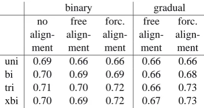
For each data source we consider 40 string com-parison algorithms. We distinguish between meth-ods with a binary comparison of n-grams and those with a gradual comparison ofn-grams (see Section 2.4). Within the category of binary meth-ods, we distinguish between three groups. In the first group, strings are compared just by counting the number of commonn-grams, ignoring the or-der of elements, see Section 2.1). In the second group the n-grams are aligned (see Section 2.2). We call this ‘free alignment’. In the third group we insist on the linguistically informed alignment ofn-grams (see Section 2.5), dubbing this ‘forced alignment’. Within the category of gradual meth-ods, we distinguish between ‘free alignment’ (see Section 2.6) and ’forced alignment’. Finally, for each of these methods, we consider both an un-normalized version of the measure as well as one normalized by length (see Section 2.3).
condi-binary gradual no free forc. free forc. align- align- align- align-
align-ment ment ment ment ment
uni 0.69 0.66 0.66 0.66 0.66
bi 0.70 0.69 0.69 0.66 0.68
tri 0.71 0.70 0.72 0.66 0.73 xbi 0.70 0.69 0.72 0.67 0.73
Table 1: Correlations between perceptual dis-tances and unnormalized string edit distance mea-surements among 15 Norwegian dialects. Higher coefficients indicate better results.
tion for validity, we check the consistency of pho-netic distance methods. For each of the meth-ods we calculated Cronbach’sα values, which is based on the average inter-correlation among the words (Heeringa, 2004, pp. 170–173). A widely-accepted threshold in social science for an accept-ableαis 0.70 (Nunnally, 1978). After the consis-tency check, we discuss validation results.
5.1 Norwegian Perception
In this section we first discuss results of unnormal-ized string edit distance measures, and will com-pare them with their normalized counterparts far-ther onwards in this section.
The Cronbach’s α values of the unnormalized measurements vary from 0.84 to 0.87. The Cron-bach’sαvalues of the methods with ‘forced align-ment’ are a bit lower than theαvalues of the other methods. An outlier arises when using the ‘forced alignment’ and gradual bigram distances:α=0.78, but these all indicate that the measurements are quite consistent.
We calculated correlations to the perceptual dis-tances which are described in Section 4.1. Re-sults are given in Table 1. Let’s note that the effect size, i.e., the r value itself, is quite high, 0.66 < r < 0.73, meaning that the various dis-tance measure are accounting for 43.6–53.3% of the variance in the perception measurements. All of the correlation coefficients are massively signif-icant (p <0.001), but given the stringency of the Mantel test, they do not differ significantly from one another.
The correlations are quite similar. The maxi-mal difference we found was0.07, so that we con-clude that none of the methods is strikingly better or worse in operationalizing the level of pronunci-ation difference that dialect speakers are sensitive
binary gradual
no free forc. free forc. align- align- align- align-
align-ment ment ment ment ment
uni 0.66 0.66 0.66 0.66 0.66
bi 0.67 0.67 0.67 0.66 0.66
tri 0.68 0.68 0.70 0.66 0.70 xbi 0.68 0.68 0.70 0.69 0.70
Table 2: Correlations between perceptual tances and different normalized string edit dis-tance measurements among 15 Norwegian di-alects. Higher coefficients indicate better results.
to.
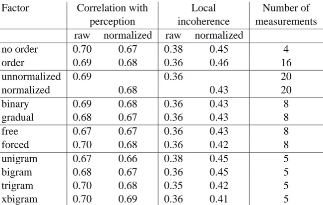
The small flood of numbers in Table 1 may seem confusing. Therefore we calculated averages per factor which are presented in Table 4. We in-vite the reader to refer to both Table 1 and Tablee 4 in following the discussion below. Table 4 shows systematic differences. For example, contextually sensitive measures (bigrams, trigrams, and xbi-grams) are usually better (and never worse) than unigram measures. The differences among the different means of operationalizing context (bi-grams, trigrams and xbigrams) seem unremark-able, however. Third, measures which are sensi-tive to linear order are slightly worse than those which are not (variants of DICE) on average5. But when comparing the first column in Table 1 with the others, we see that the highest correla-tions (0.73) are found among the order sensitive methods. Fourth, forcing alignment to respect vowel/consonant differences yields a modest im-provement in scores. Fifth, we see no clear ad-vantage in measurements which weight n-grams more sensitively to those binary comparison meth-ods which distinguish only same and different.
Sixth, and most surprisingly, we can compare Table 1 which provides the correlation of edit dis-tances which were not normalized for length, with Table 2, which provides the results of the mea-surements which were normalized. For some nor-malized measurements the Cronbach’sαvalue are minimally higher (0.01). But comparison of the correlation coefficients shows that normalization never improves measurements, and often leads to a deterioration. In Table 4 averages for the normal-ized measurements are given. Normalnormal-ized
mea-5When using the unnormalized versions of the ‘DICE’
binary gradual no free forc. free forc. align- align- align- align-
align-ment ment ment ment ment
uni 0.41 0.37 0.37 0.37 0.37
bi 0.37 0.35 0.37 0.36 0.35
tri 0.37 0.33 0.35 0.36 0.35 xbi 0.36 0.35 0.35 0.37 0.35
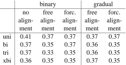
Table 3: Local incoherence values based on travel distances for the unnormalized string edit dis-tance measurements between 15 Norwegian di-alects. The lower the local incoherence value, the better the measurement technique.
surements display the same systematic differences that unnormalized measurements show, except for the differences between methods which consider the order of segments and methods which do not. Measures which are sensitive to linear order are slightly better than those which are not (variants of DICE).
5.2 Norwegian Geographic Sensitivity
As we mentioned in Section 4.2, Norway is very rugged. Therefore we based our local incoher-ence values on travel distances rather than on ge-ographic distances “as the crow flies”. We com-puted local incoherence values for both unnormal-ized and normalunnormal-ized string edit distance measure-ments. The comparison confirms the findings of Section 5.1: unnormalized methods always per-form better than normalized ones. The unnormal-ized results are presented in Table 3.
Recall that lower local incoherence values should reflect better measurement techniques. When we examine the table as a whole, we note again that the various techniques are not hugely different—they perform with similar degrees of success.
In Table 4, we find average local incoherence values for the factors under investigation. We find first that contextually sensitive measures (bigrams, trigrams, and xbigrams) are again superior to un-igram methods, and second, measures which are sensitive to linear order are superior to the DICE-like methods (unnormalized versions). Third, lin-guistically informed alignments, which respect the vowel/consonant distinction, perform better than uninformed (“free”) alignment (for the normalized versions). Fourth, the average values do not
sug-gest any benefit to the gradual weighting of n -grams in comparison with the binary weighting. Most surprisingly, normalization again appears to have a deleterious effect on the probity of the mea-surements.
We must stress again that these finer interpreta-tions results require confirmation with a larger set of sites.
5.3 German Geographic Sensitivity
When checking the consistency of the German measurements we find Cronbach’s α values of 0.95 and 0.96 for all methods without alignment or with ’free alignment’ and for all unigram based methods. The higher Cronbach’sα levels for this data set reflect the fact that it is larger. We find lowerαvalues of 0.83–0.85 for the methods with ‘forced alignment’. This accords with the consis-tency results for the Norwegian measurements.
When using bigrams,αis equal to0.80(binary, normalized),0.51(gradual, normalized),0.74 (bi-nary, unnormalized) and0.45(gradual, unnormal-ized). These low values are striking, and we found no explanation for them, but they suggest that we should not attach much significance to this combi-nation of measurement properties. On average, the unnormalizedα’s are the same as the normalized
α’s.
Since consistency values are higher than 0.70 (with one exception), we validated the methods by calculating the geographic local incoherence val-ues. We would have preferred to use perceptions, but we have no such data in the German case.
Since we found unnormalized string edit dis-tance measurements superior to normalized ones in the Sections 5.1 and 5.2, we focus in this sec-tion on the unnormalized methods. Unnormalized results are shown in Table 5.
Recall that the lower the local incoherence value, the better the measurement technique. We include this table for the sake of completeness, but it is clear that the results do not jibe with the re-sults obtained from the Norwegian data. Unigram-based processing appears to be superior, and con-text inferior; order-sensitive processing is inferior to order-insensitive processing, and linguistically informed (“forced”) alignment appears to offer no advantage.
Factor Correlation with Local Number of perception incoherence measurements raw normalized raw normalized
no order 0.70 0.67 0.38 0.45 4
order 0.69 0.68 0.36 0.46 16
unnormalized 0.69 0.36 20
normalized 0.68 0.43 20
binary 0.69 0.68 0.36 0.43 8
gradual 0.68 0.67 0.36 0.43 8
free 0.67 0.67 0.36 0.43 8
forced 0.70 0.68 0.36 0.42 8
unigram 0.67 0.66 0.38 0.45 5
bigram 0.68 0.67 0.36 0.45 5
trigram 0.70 0.68 0.35 0.42 5
xbigram 0.70 0.69 0.36 0.41 5
Table 4: Average correlations between perceptual distances and raw, i.e., unnormalized string edit dis-tance measurements among 15 Norwegian dialects. Higher coefficients and lower local incoherence values indicate better results.
binary gradual
no free forc. free forc. align- align- align- align-
align-ment ment ment ment ment
uni 0.94 0.88 0.87 0.88 0.87
bi 1.00 0.98 2.09 0.92 5.71
tri 1.09 1.05 2.45 0.93 2.09 xbi 0.96 0.95 2.45 0.98 2.45
Table 5: Local incoherence values based on geo-graphic distances for for the unnormalized string edit distance measurements 186 German dialects. The lower the local incoherence value, the better the measurement technique.
rather more confidence in the Norwegian than in the German results. This is due on the one had to the availability of independently behavioral data we can use to independently validate our compu-tations, but also to the more stable set of values we see in the case of the Norwegian data. Exactly why the German data is so much more variable is also a question we must postpone to future work.
6 Conclusions and Prospects
In this paper we examined a range of string com-parison algorithms by applying them to Norwe-gian and German dialect comparison. The Nor-wegian results suggest that sensitivity to linguis-tic context in the form ofn-grams, and to linguis-tic structure in alignment improves measurement
techniques, but they do not confirm the value of differential weighting for n-grams. The results mostly suggest that sensitivity to order of seg-ments improves the measureseg-ments.
The larger German data likewise is unfortu-nately more recalcitrant (as are other data sets we have examined, but in which we have less confi-dence). A disadvantage of the German data may be that several transcribers were involved, work-ing over a period of twenty years, and that two types of surveys were used, having different or-ders of sentences. There may be subtle differences in pronunciation as a result of subjects’ becoming more relaxed or more impatient in the course of a survey interview.
On the other hand, the Norwegian data set is small (15 dialect sites). Our conclusions rely on assumptions of its quality and transcriber consis-tency, but this warrants further examination. We also cannot exclude the possibility that optimal measurements depend on features of the language and/or data set.
must keep this in mind.
Acknowledgments
We are grateful to Therese Leinonen, Jens Moberg and Jelena Prokiˇc for comments on this work, and in particular for their suggestion that one should also examine the length normalization. We also thank the workshop reviewers, in particularly one who was productively harsh about the treatment of normalization in an earlier version, and also pointed out literature we had insufficiently taken note of. Finally, we are indebted to the Nether-lands Organization for Scientific Research, NWO, for support (project “Determinants of Dialect Vari-ation, 360-70-120, P.I. J. Nerbonne)
References
Eric Bonnet and Yves Van de Peer. 2002. zt: A soft-ware tool for simple and partial Mantel tests.
Jour-nal of Statistical Software, 7(10):1–12. Available
via:http://www.jstatsoft.org/.
Hans Goebl. 1982. Dialektometrie: Prinzipien und Methoden des Einsatzes der Numerischen Taxonomie im Bereich der Dialektgeographie.
¨
Osterreichische Akademie der Wissenschaften, Wien.
Hans Goebl. 1984. Dialektometrische Studien:
An-hand italoromanischer, r¨atoromanischer und gal-loromanischer Sprachmaterialien aus AIS und ALF. 3 Vol. Max Niemeyer, T¨ubingen.
Charlotte Gooskens. Traveling time as a predictor of linguistic distance. Dialectologia et Geolinguistica. submitted, 3/2004.
Charlotte Gooskens and Wilbert Heeringa. 2004. Per-ceptual evaluation of Levenshtein dialect distance measurements using Norwegian dialect data.
Lan-guage Variation and Change, 16(3):189–207.
Joachim G¨oschel. 1992. Das Forschungsinstitut f¨ur Deutsche Sprache “Deutscher Sprachatlas. Wis-senschaftlicher Bericht, Das Forschungsinstitut f¨ur Deutsche Sprache, Marburg.
Wilbert Heeringa. 2004. Measuring Dialect
Pronunci-ation Differences using Levenshtein Distance. Ph.D.
thesis, Rijksuniversiteit Groningen.
Cor Hoppenbrouwers and Geer Hoppenbrouwers. 2001. De indeling van de Nederlandse streektalen:
Dialecten van 156 steden en dorpen geklasseerd vol-gens de FFM (feature frequentie methode).
Konin-klijke Van Gorcum, Assen.
Diana Inkpen, O. Frunza, and Grzegorz Kondrak. 2005. Automatic Identification of Cognates and
False Friends in French and English. In Galia An-gelova, Kalina Bontcheva, Ruslan Mitkov, Nicolas Nicolov, and Nicolai Nicolov, editors, International
Conference Recent Advances in Natural Language Processing, pages 251–257, Borovets.
Brett Kessler. 1995. Computational dialectology in Irish Gaelic. In Proc. of the European ACL, pages 60–67, Dublin.
Brett Kessler. 2005. Phonetic comparision algo-rithms. Transactions of the Philological Society,
103(2):243–260.
Grzegorz Kondrak. 2005. N-gram similarity and dis-tance. In Proceedings of the Twelfth International
Conference on String Processing and Information Retrieval (SPIRE 2005), pages 115–126, Buenos
Aires, Argentina.
Joseph Kruskal. 1999. An overview of sequence com-parison. In David Sankoff and Joseph Kruskal, edi-tors, Time Warps, String Edits and Macromolecules:
The Theory and Practice of Sequence Comparison,
pages 1–44. CSLI, Stanford. 11983.
Andr´es Marzal and Enrique Vidal. 1993. Computation of normalized edit distance and applications. IEEE
Transactions on Pattern Analysis and Machine In-telligence, 15(9):926–932.
John Nerbonne and Peter Kleiweg. 2003. Lexical vari-ation in LAMSAS. Computers and the Humani-ties, 37(3):339–357. Special Iss. on Computational
Methods in Dialectometry ed. by John Nerbonne and William Kretzschmar, Jr.
John Nerbonne and Peter Kleiweg. 2006. Toward a dialectological yardstick. Quantitative Linguistics, 13. accepted.
Jum C. Nunnally. 1978. Psychometric Theory.
McGraw-Hill, New York.
Jean S´eguy. 1973. La dialectometrie dans l’atlas lin-guistique de gascogne. Revue de Linlin-guistique