DOI: 10.1534/genetics.108.098913
Binary Trait Mapping in Experimental Crosses With Selective Genotyping
Ani Manichaikul*
,1and Karl W. Broman
†*Department of Biomedical Engineering, University of Virginia, Charlottesville, Virginia 22908 and†Department of Biostatistics and Medical Informatics, University of Wisconsin, Madison, Wisconsin 53706
Manuscript received November 19, 2008 Accepted for publication April 21, 2009
ABSTRACT
Selective genotyping is an efficient strategy for mapping quantitative trait loci. For binary traits, where there are only two distinct phenotypic values (e.g., affected/unaffected or present/absent), one may consider selective genotyping of affected individuals, while genotyping none or only some of the unaffecteds. If selective genotyping of this sort is employed, the usual method for binary trait mapping, which considers phenotypes conditional on genotypes, cannot be used. We present an alternative approach, instead considering genotypes conditional on phenotypes, and compare this to the more standard method of analysis, both analytically and by example. For studies of rare binary phenotypes, we recommend performing an initial genome scan with all affected individuals and an equal number of unaffecteds, followed by genotyping the full cross in genomic regions of interest to confirm results from the initial screen.
W
E consider the problem of mapping genetic loci contributing to a binary trait in an experimental cross with selective genotyping. There are two clear approaches for linkage analysis with a binary trait. Typically, we compare the proportion of affected individuals across genotype groups (Xu and Atchley1996). Alternatively, we can compare genotype fre-quencies between affected and unaffected individuals, similar to Henshall and Goddard (1999). Beyond
these two basic approaches, binary trait mapping has seen fundamental advances in regression models (McIntyre et al. 2001; Deng et al. 2006), extensions
to multiple-QTL mapping (Coffmanet al.2005; Chen
and Liu 2009), and the development of Bayesian
algorithms (Yi and Xu 2000; Huang et al. 2007).
However, the original data structure and approach have remained intact. Existing methods for binary trait mapping largely require the availability of genotype and phenotype data for a representative sample of both affected and unaffected individuals, and we have not yet seen a well-developed framework for binary trait mapping in the presence of selective genotyping.
It is not uncommon to see genotype data on affected individuals only, in which case the above methods cannot be used. Instead, we can compare observed genotype frequencies to the expected segregation ratios given the cross type, in a test for segregation distortion (see Faris et al. 1998; Lambrides et al. 2004). For
example, the expected segregation proportions for an intercross are 1:2:1. The observed genotypes can then
be described by a multinomial model, and statistically significant deviation from the expected segregation ratios among the genotyped affected individuals would suggest genotype–phenotype association. Gene map-ping approaches that model genotypes rather than phenotypes have been developed extensively in the analysis of affected human relative pairs (see, for example, Risch 1990; Holmans 1993; Hauser and
Boehnke1998). In the analysis of experimental crosses,
however, this type of approach has been developed primarily for the identification of monogenic mutants (Moranet al.2006).
Once all affected individuals are genotyped, an in-vestigator may go on to genotype unaffected individuals. With this genotyping strategy in mind, we present several potential methods of analysis that might be applied in this context. First, we consider a standard analysis of the genotyped individuals, with disease proportions compared across genotype groups (Xu
and Atchley 1996). Having omitted ungenotyped
individuals, this method of analysis appears invalid because the estimated disease proportions are biased upward, reflecting an overrepresentation of affecteds in the set of genotyped individuals under consideration. As an alternative, we develop a reverse approach with genotype frequencies compared across phenotype groups. Because selective genotyping does provide a representative sample of genotypes for each phenotype group, this reverse approach does not face the bias in parameter estimation seen with the standard approach. We further extend the reverse approach to incorporate a segregation assumption, as is necessary for an affec-teds only analysis. Finally, we present a full-likelihood analysis accounting for selective genotyping, similar to
1Corresponding author:Department of Biomedical Engineering, Univer-sity of Virginia, Box 800759, Health System, Charlottesville, VA 22908. E-mail: [email protected]
that suggested by Lander and Botstein (1989) for
quantitative traits. We develop the full-likelihood ap-proach both with and without incorporating an assump-tion on the genotype segregaassump-tion proporassump-tions.
Having put forth each of these methods, we derive analytic relationships among them. These relationships provide important insight regarding application of the presented methods under selective genotyping. Most notably, we find that making a segregation assumption can lead to spurious evidence of a QTL, but is necessary to treat the case of affecteds only genotyping. We demonstrate properties of the methods in an analysis of recovery from infection by Listeria monocytogenes in intercross mice and further compare power of the methods through computer simulations. Finally, we synthesize our analytical and simulation results to offer more general suggestions for the analysis of binary trait data with selective genotyping.
METHODS
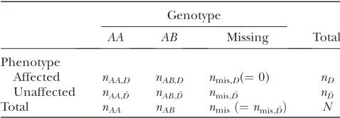
For simplicity, we present methods for the case of a backcross. For analysis, we consider backcross data consisting of binary phenotypes (affected or unaf-fected) for all individuals and marker genotypes (AA or AB) on all affecteds and all, some, or none of the unaffecteds. We present methods of analysis to address these three genotyping strategies for binary trait data. The observed data are represented in Table 1.
Throughout our description of the methods, we use the following notation. LetN be the total number of individuals in the cross, withnobsgenotyped individuals andnmis¼Nnobsungenotyped individuals. We assign the indexesi¼1,. . .,Nsuch that individualsi2{1,. . ., nobs} are genotyped, and the remaining individuals are ungenotyped. Let Di ¼ 1 or 0 according to whether
individualiis affected or unaffected. We takeGi2{AA,
AB} to denote the underlying unobserved genotype at the putative QTL of interest, whileOmi 2{AA,AB,}
denotes the observed genotype at markerm, with ‘‘’’ indicating a missing value.
Standard approach: In dealing with selective geno-typing, one possible approach is to ignore individuals
without genotype data, performing an analysis of genotyped individuals only. Once we have omitted individuals with missing genotypes from our analysis, we can use the approach of Xuand Atchley(1996) to
look for genotype–phenotype association by testing for a difference in disease probability across genotypes.
LetpAA¼Pr(Di ¼1jGi¼AA) andpAB¼Pr(Di¼
1jGi¼AB) denote the penetrance values (the
condi-tional phenotype probabilities given the genotype at a putative QTL), and let p ¼ Pr(Di ¼ 1) denote the
marginal phenotype probability (i.e., the prevalence of disease).
Similar to standard interval mapping for quantitative traits (Landerand Botstein1989), the approach of Xu
and Atchley(1996) makes use of the conditional QTL
genotype probabilities given the full set of multipoint marker data for theith individual,pig¼Pr(Gi¼gjOi).
By convention, evidence against the null hypothesis of genotype–phenotype independence, Pr(DjG)¼Pr(D), in favor of the alternative hypothesis of a QTL, Pr(DjG)6¼ Pr(D), is presented as the log10-likelihood ratio
LODF¼log10
maxpAA;pABPrðDjO;pAA;pABÞ
maxpPrðD;pÞ
¼log10
Q i
P
g2fAA;ABg½pig ðpˆgÞDi ð1pˆgÞ1Di Q
iðpˆÞDi ð1pˆÞ1Di
( )
;
where we model affection status as a Bernoulli random variable with a common probability under the null and with genotype-specific probabilities under the alterna-tive hypothesis. Assuming no missing genotype data for reasons other than the selective genotyping, and no genotyping error, the maximum-likelihood estimates (MLEs) at the markers are simply sample proportions. Between markers, we can perform interval mapping by an EM algorithm (Dempster et al. 1977), which has
been previously described for this application (Xuand
Atchley1996; Broman2003).
The forward approach using LODFis appropriate in the case that we have genotyped all individuals. How-ever, if we have done selective genotyping with regard to phenotypes, the approach will yield biased and incon-sistent estimates ofpAAandpAB. As a result, the validity of this approach for selective genotyping is not imme-diately apparent.
Reverse approach, conditioning on phenotypes: As an alternative, we can also look for genotype–phenotype association by reversing the standard approach and instead modeling genotypes conditional on pheno-types. This approach is technically quite similar to the logistic regression model presented by Henshalland
Goddard(1999), but we present it in a framework that
elucidates its relationship with the standard approach of Xuand Atchley(1996). Placing the reverse approach
in this likelihood framework also allows it to be easily adapted for analysis of affecteds only, as will be seen
TABLE 1
Data at a single genetic marker from a backcross experiment with binary phenotypes
Genotype
AA AB Missing Total
Phenotype
Affected nAA,D nAB,D nmis,D(¼0) nD
Unaffected nAA;D˜ nAB;D˜ nmis;D˜ nD˜
Total nAA nAB nmisð¼nmis;D˜Þ N
below. Again, we consider only genotyped individuals and omit the rest from our analysis.
Let fD ¼ Pr(Gi ¼ AA j Di ¼ 1) and fD˜ ¼PrðGi¼
AAjDi¼0Þdenote the affection-status-specific
proba-bilities of the AA genotype at the putative QTL of interest, and letf¼Pr(Gi¼AA) denote the marginal
probability of the AA genotype. (For an intercross, we must handle the three possible genotypes {AA,AB, BB}, and so we would consider the vector f¼
PrðGi¼AAÞPrðGi¼ABÞ
½ T and analogous vectors for
fDandfD˜.)
We calculate the LOD score measuring support for a QTL as the log10-likelihood ratio comparing evidence for the alternative hypothesis, Pr(Dj G)6¼Pr(D) [or equivalently, Pr(GjD) 6¼Pr(G)], in favor of the null hypothesis of independence. Here, we model genotypes at the putative QTL using a Bernoulli process (or multinomial for an intercross) with a common proba-bility under the null and with disease-status-specific probabilities under the alternative hypothesis (see Table 2).
To allow analysis at both marker and nonmarker locations, we perform interval mapping using an EM algorithm to calculate the necessary MLEs. Analogous to thepigfor standard interval mapping, we make use of
the reverse quantities,qig¼Pr(OijGi¼g), probabilities
of the full set of observed marker data given a specified value of the underlying QTL genotype, g. We have developed hidden Markov models to obtain the qig;
details are provided inappendix a.
Reverse approach, modified: Having presented the reverse approach above, a simple modification allows us to incorporate knowledge regarding the structure of the cross. In particular, we may specify the null hypothesis value offto be 12 for a backcross (or f¼ 14 12
T
for an intercross). This prior knowledge is crucial in the analysis of affecteds only, for which it is infeasible to simply check for a difference in genotype proportions across phenotype groups, as was done above.
Here, the modified LOD score, LODR;seg¼log10 maxfD;fD˜PrðO jD;fD;fD˜Þ=PrðO;f¼
1 2Þ
, quanti-fies evidence for segregation distortion,i.e., deviation of observed genotype counts from their expected distri-bution. In an affecteds only analysis, this view of evidence suggests genotype–phenotype association and so indicates the presence of a QTL.
Since the alternative hypothesis remains the same as in the original reverse approach, LODR, the MLEs for
fDandfD˜may be obtained in the same way as described
above. Note that a reasonable approach to take with this method is to constrain the conditional geno-type probabilities such that their weighted average,
fDp1fD˜ ½1p, is equal to the marginal genotype
probability,f. However, we use the unconstrained value
in calculating LODR,seg, incorporating the constraint through a full-likelihood analysis developed further below.
Full-likelihood analysis: Performing a full-likelihood analysis allows us to forgo conditioning on either genotypes or phenotypes. Conceptually, this model makes complete use of the available data in assessing evidence of a QTL. An apparent advantage of this approach is that ungenotyped individuals can be in-cluded in the likelihood. However, careful examination in theresultsbelow shows that full-likelihood analysis
yields results quite similar to those of both the forward and reverse approaches.
The full-likelihood function models the joint proba-bility of disease status and observed genotypes. We write the full likelihood of a QTL at the putative site of interest in terms of parametersfD,fD˜, andpas
likðfD;fD˜;pÞ ¼
YN
i¼1
PrðDi;Oi;fD;fD˜;pÞ
¼likðfD;fD˜jDÞ likðpÞ: ð1Þ
Since the full likelihood can be decomposed into orthogonal components to separatefDandfD˜ fromp
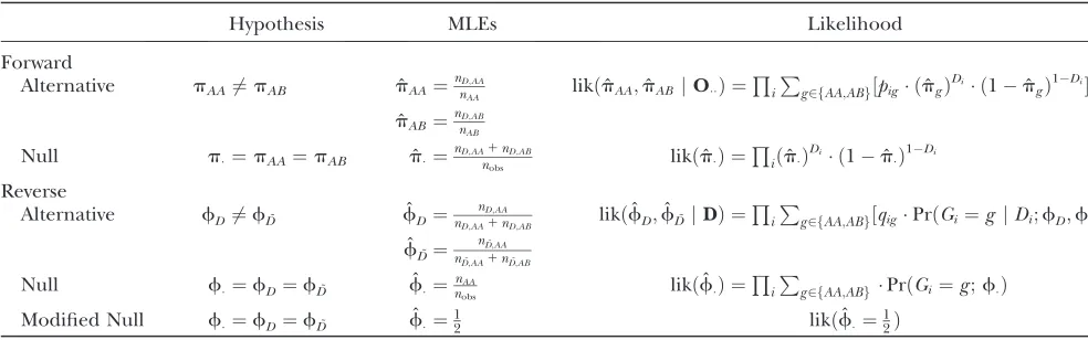
TABLE 2
Summary of forward and reverse approaches and likelihood functions
Hypothesis MLEs Likelihood
Forward
Alternative pAA6¼pAB pˆAA¼nD
;AA
nAA likðpˆAA;pˆABjOÞ ¼
Q i
P
g2fAA;ABg½pig ðpˆgÞ
Di ð1pˆ
gÞ
1Di
ˆ pAB¼
nD;AB
nAB Null p¼pAA¼pAB pˆ¼nD;AA
1nD;AB
nobs likðpˆÞ ¼
Q
iðpˆÞDi ð1pˆÞ1Di
Reverse
Alternative fD6¼fD˜ fˆD ¼ nD;AA
nD;AA1nD;AB likð ˆ
fD;fˆD˜ jDÞ ¼ Q
i P
g2fAA;ABg½qigPrðGi¼g jDi;fD;fD˜Þ
ˆ fD˜¼
nD˜;AA
nD˜;AA1nD˜;AB
Null f¼fD¼fD˜ fˆ¼nnobsAA likð
ˆ
fÞ ¼QiPg2fAA;ABgPrðGi¼g;fÞ
Modified Null f¼fD¼fD˜ fˆ¼12 likðfˆ¼12Þ
(see appendix b for details), the resulting MLEs are
simply those obtained by performing the maximization separately. At the markers, these are again the appro-priate sample averages as specified in the previous sections above. Estimating the position of a QTL does not depend on the value p since this parameter
estimate is fixed across the genome.
Constrained full likelihood:Analogous to the modified reverse approach that incorporates evidence for segre-gation distortion, we can also perform full-likelihood analysis under the assumption that marginal genotype probabilities should follow their null segregation values. The resulting full-likelihood function is the same as that specified above, but subject to the constraint that disease-status-specific genotype probabilities average to a marginal value off¼1
2. We write this constraint in terms of the overall probability of disease,p:
f¼fDp1fD˜ ½1p ¼
1
2: ð2Þ
(For the case of an intercross, f¼ 1 4 1 2
T
, so the equation above becomes a two-component constraint.) Analysis is performed using allNindividuals in the cross, both genotyped and ungenotyped. The constrained full-likelihood LOD score is written as
LODNFull;seg¼log10
maxfD;fD˜;pjf¼1=2likðfD;fD˜;pÞ
maxplikðf¼1=2;pÞ
:
Under the null hypothesis, the MLE ˜p¼nD=N is the
same as in the absence of the constraint, while ˜f¼1 2 according to the segregation assumption. To maximize the constrained likelihood under the alternative hy-pothesis, we use an EM algorithm, described in appen-dix c.
Significance thresholds: After performing a genome scan using any of the methods presented above, we can make use of significance thresholds in reporting statis-tical significance for genomic regions of interest. The significance thresholds must account for multiple comparisons arising in the complete genome scan. A typical way to perform this adjustment while controlling the rate of detecting false positive QTL is to examine the distribution of the genomewide maximum LOD score under the global null hypothesis of no QTL.
For standard interval mapping, significance thresh-olds conditioning on observed genotypes and pheno-types may be obtained empirically by permutation (Churchilland Doerge1994), shuffling phenotypes
while keeping genotypes fixed to approximate the null distribution of the genomewide maximum LOD score. In the case of methods incorporating a segregation assumption, such as LODR,seg, it may not make sense to condition on observed genotypes. For example, in an affecteds only analysis, the observed genotypes contain
all of the information we use to test for linkage. If we condition on those observed genotypes in calculating the null distribution, we effectively condition out any evidence in the data. Put more simply, we cannot shuffle phenotypes in an affecteds only analysis because all individuals have the same phenotype. Instead, we can estimate the null distribution by simulation using a gene-dropping approach (MacCluer et al. 1986) to
simulate new genotypes preserving the cross structure and pattern of missing genotypes from the original data set. The resulting significance thresholds are reported conditional on observed phenotypes, while averaging across possible sets of genotypes given the cross used to generate the data. Since the simulation-based signifi-cance thresholds do not condition on the observed genotypes, they are appropriate for analyses in which we have incorporated evidence for segregation distortion or deviation from expected segregation ratios. We describe this form of evidence more explicitly in the
resultsbelow.
RESULTS
We have presented approaches to calculating like-lihoods and corresponding likelihood ratios to assess genotype–phenotype association for binary trait map-ping in the presence of selective genotymap-ping. Since all of these methods are likelihood based, they are closely related. In this section, we highlight key relationships between the various approaches. We summarize all presented relationships at the end of this section.
Reverse approach vs. modified reverse approach: There is a direct relationship between LODR, in which we use the MLE ˆfto calculate the null likelihood, and LODR,seg, in which we assumef¼12 according to the
expected genotype frequencies in a backcross,
LODR;seg¼log10 lik
ðfˆD;fˆD˜jD;OmÞ
likðf¼1 2jOmÞ
( )
¼log10
likðfˆD;fˆD˜jD;OmÞ
likðfˆjOmÞ
3 likðfˆjOmÞ
likðf¼1 2;OmÞ
( )
¼LODR1LODseg:dist:;
where LODseg:dist:¼log10 likðfˆjOmÞ=likðf¼12jOmÞ
quantifies evidence for segregation distortion or de-viation of the observed genotypes from the assumed segregation proportion,f¼1
2.
Full likelihoodvs.reverse approach:Let LODnobs
Full be the full-likelihood LOD score based on genotyped individuals only and LODN
decomposed as a product of the likelihood for parame-ters fD;fD˜ and the likelihood for p, as shown in (1)
above. So, we can factor out the likelihood for phenotype probability from the full likelihood to relate it back to the reverse approach. Because this factorization applies at both marker and nonmarker locations, the relationship LODnobs
Full¼LODNFull¼LODRholds quite generally even in the presence of missing genotype data or genotyping error (seeappendix dfor details).
Forward vs. reverse approach: The forward and reverse methods of analysis are closely related as they are both likelihood-ratio-based tests of independence. For the case of no missing genotypes or genotyping error, we can examine the relationship analytically at marker locations
LODF ¼log10
PrðDjO;pˆAA;pˆABÞ
PrðD;pˆÞ
¼log10 PrðDjO;pˆAA;pˆABÞ PrðO;fˆÞ PrðD;pˆÞ PrðO;fˆÞ
ð¼LODnobs
FullÞ
¼LODR;
where the estimated parameters ˆpAA;pˆAB, and ˆfare the
MLEs as specified in themethodssection above. Note
that these relationships apply only at marker locations, in the case of no missing genotypes. It is in this special case that all MLEs are obtained as sample averages, and so the computed likelihood ratio is the same whether conditional on genotypes or phenotypes. At nonmarker locations, we must employ the relationships in (A6) to obtain the full-likelihood MLEs, ˆpAA;pˆAB, and ˆf, so
these values could differ from those obtained by the standard approach, LODF.
Overall relationships:Here, we summarize the rela-tionships among the proposed methods presented here, together with those shown inappendix d. At the
markers we have the following relationships:
LODnobs
Full¼LODF¼LODR LODR;seg¼LODF1LODseg:dist::
The following relationships hold more generally at both marker and nonmarker locations:
LODnobs
Full¼LODNFull¼LODR
LODNFull;seg#LODR;seg¼LODR1LODseg:dist:
That LODRagrees with full-likelihood analysis, whether or not we include ungenotyped individuals in the analysis, suggests it is unnecessary to perform full-likelihood analysis, since we can get the exact same results using the simpler reverse approach. However, we also see that the modified reverse approach incorpo-rates evidence for segregation distortion, which can be
irrelevant to linkage if we have genotyped both affecteds and unaffecteds. Hence, full-likelihood analysis may still be necessary to incorporate the segregation assumption while avoiding spurious evidence, as in LODN
Full;seg.
APPLICATION
To demonstrate features of our proposed methods, we perform analysis of recovery from L. monocytogenes infection in 116 mice from an intercross of the resistant strain C57BL/6ByJ and the susceptible strain BALB/ cByJ (Boyartchuk et al. 2001), using the data set
available in the R/qtl package (Broman et al. 2003).
In our analysis, we make use of genotypes at 131 genetic markers on the 19 autosomes. Although phenotypes were recorded as survival times in the original study, we converted them to binary values to demonstrate appli-cation to our proposed methods. (Note that analyzing survival data as binary values is only one possible strategy in handling survival data; see Broman2003 for a more
complete treatment of this particular data set.) Accord-ingly, binary phenotypes were calculated to indicate whether or not mice survived to 264 hr following infection. Among the 116 phenotyped mice in this data set, 35 survived and 81 died within 264 hr. Since survival is the rarer phenotype in this cross, we refer to the 35 survivors as affected individuals. With the full data, an appropriate analysis would use the standard approach, LODF, with the available full genotypes. To explore the set of possible genotyping strategies using real data, we subset the available genotypes to create two additional versions of this data set for analysis: one data set with genotypes on affecteds only and another with equal numbers of affecteds and unaffecteds genotyped. In each case, we apply methods of analysis appropriate for the genotyping strategy at hand.
Since some of the presented methods are sensitive to segregation distortion, we note in advance that chro-mosome 13 showed the strongest evidence of overall deviation from the expected genotype proportions. In particular, the marker D13M233 had genotype segrega-tion proporsegrega-tions of 40:41:21 rather than the expected 1:2:1, giving a segregation distortion LOD score of 2.97 (P ¼ 0.097 by gene-dropping simulation with 10,000 replicates). In contrast, the marker D2M365 on chro-mosome 2 showed little segregation distortion, with segregation proportions of 24:59:27 and a segregation distortion LOD score of 0.12.
Standard analysis: We first consider a standard analysis with full genotypes. In this case, it is appropriate to perform standard interval mapping using the forward approach, LODF, conditioning phenotypes on geno-types. In calculating our LOD curve, we use an EM algorithm, as implemented in R/qtl (Broman et al.
Doerge 1994) to assign statistical significance and
obtain (with 10,000 permutation replicates) a 5% significance threshold of 3.57.
The LOD curve (Figure 1) has statistically significant peaks on chromosomes 5 and 13, with corresponding P-values of,0.001 and 0.042, respectively. The evidence seen on chromosome 13 is not influenced by segrega-tion distorsegrega-tion and shows that genotype proporsegrega-tions differ significantly by affection status.
Affecteds only analysis: If only the 35 affected individuals were genotyped, the forward and reverse approaches, LODF and LODR, respectively, are not appropriate because they will always produce LOD scores of strictly zero. Instead, we calculate the LOD curve using the reverse approach, LODR,seg, making use of the intercross segregation assumption, with geno-typesCC,CB, andBBsegregating according to the ratios 1:2:1. A 5% significance threshold is calculated by simulation to be 3.57.
The LOD peak on chromosome 5 (Figure 1) is statistically significant with a LOD score of 4.07 (P ¼ 0.019). To follow up on this result, it is appropriate to obtain genotypes for the full cross at the peak position on chromosome 5. In our follow-up analysis of D5M357,
we test for a difference in genotype proportions across affected and unaffected individuals. Among affected individuals, the observed genotype distribution was 18:16:1, compared to 12:39:30 among unaffecteds, yielding an exact pointwise P-value of 2.93 106. On
the basis of this analysis, we conclude there is evidence for a QTL on chromosome 5, and the significant result obtained using affecteds only was not driven by spurious segregation distortion.
Although there was good evidence of a QTL on chromosome 13 using full genotypes, we detected no evidence of a QTL on chromosome 13 using affecteds only (maximum LOD score of 1.25, P . 0.99). The results on chromosome 13 demonstrate that the reverse approach, LODR,seg, provides reliable results only when there is little segregation distortion in the overall set of genotypes. In this particular data set, there was strong segregation distortion among the pooled set of affec-teds and unaffecaffec-teds, while affected individuals alone had genotype proportions close to their null values.
Equal numbers of affecteds and unaffecteds geno-typed:By genotyping both affecteds and unaffecteds, we no longer require the use of a segregation assumption and so can avoid the problem of distorted evidence that we encountered in our affecteds only analysis. Here, we consider the same intercross as above, but now we have genotyped 35 unaffected mice (selected at random), in addition to the 35 affected individuals. In this case, we perform analysis using the reverse approach, LODR, and use permutation to get a 5% significance threshold of 3.65.
The profile of our observed LOD curves (Figure 1) is very similar to that obtained by standard analysis with complete genotyping. The overall strength of the signal obtained by partial genotyping is somewhat attenuated, but we still have reasonable evidence of QTL on chromosome 5 and 13, withP-values 0.085 and 0.026, respectively. After the initial genome scan using this portion of the cross, we recommend following up with genotypes on the full cross in genomic regions of interest. For example, on chromosome 5 we find that the remaining unaffected individuals show D5M357 genotype proportions of 5:21:20, compared to 7:18:10 among the first 35 genotyped unaffecteds. These results confirm that the unaffecteds overall have a relatively larger proportion of homozygote BB individuals and smaller proportion ofCCindividuals. Further, the peak positions obtained by our partial genotyping strategy are identical to those obtained by analysis of the full cross. Thus, genotyping an equal number of affected and unaffected individuals combined with follow-up using the full cross provides an effective way to locate QTL while vastly reducing the amount of genotyping required.
To examine sensitivity of our results to randomness in the set of unaffected individuals selected for genotyp-ing, we repeated the analysis with 100 different sets of 35 Figure 1.—Analysis of intercross data from Boyartchuk
et al.(2001) with significant results on chromosomes 5 and 13, and chromosome 2 shown for comparison. LOD curves are generated using four different methods and normalized by their corresponding 5% significance thresholds for com-parison: (i) The LOD with full genotypes is calculated by stan-dard interval mapping according to the method of Xu and
Atchley (1996) (shaded line), with a 5% permutation
threshold of 3.57; (ii) with genotypes on affecteds only, the LOD curve is calculated by the reverse approach using an in-tercross segregation assumption, LODR,seg (dashed shaded line), and the appropriate 5% simulation threshold is 3.57; (iii) using genotypes on 35 unaffecteds and all 35 affecteds, the LOD curve is calculated by the reverse approach, LODR (solid line), with a corresponding 5% permutation threshold of 3.65; and (iv) using genotypes on 35 unaffecteds and all 35 affecteds, the LOD curve is calculated by the full likelihood with the segregation assumption, LODN
randomly selected unaffected mice. We saw qualitatively similar results across this set of replicates, with reason-able evidence of QTL on chromosomes 5 and 13 in the majority of samples (results not shown). This investiga-tion suggests genotyping all affecteds and an equal number of unaffecteds is an effective way to capture evidence of QTL in the full cross, while genotyping only a fraction of the individuals.
Some unaffecteds genotyped using constrained maximum likelihood: Incorporating a segregation as-sumption is most useful for affecteds only analysis, where we have zero power to map QTL without such an assumption. Here, we consider incorporating this assumption in the more moderate case of selective genotyping with equal numbers of affecteds and un-affecteds genotyping.
We examine the same set of genotyped individuals as above, with genotypes on 35 unaffecteds and all 35 affected individuals, and perform analysis with the inclusion of a segregation assumption. Toward this end, both the reverse approach and the full likelihood are possible options to accommodate the assumption. How-ever, as shown inresultsabove, LODR,segis equivalent
to a standard analysis, plus the LOD for segregation distortion. In mapping QTL, we are generally not in-terested in overall segregation distortion. We perform analysis by LODN
Full;seg to eliminate the possibility of spurious evidence. Since we have eliminated evidence for segregation distortion, we use permutation, rather than simulation, to obtain a 5% significance threshold of 3.56. The overall shape of the LOD curve produced by this approach agrees quite closely with the full and partial genotyping results shown in Figure 1. Still, we do note differences that reflect properties of the methods. The peak on chromosome 5 shows a LOD score of 4.06 (P¼ 0.018), greater than the value of 3.37 using the reverse approach. On the other hand, the peak evidence on chromosome 13 using LODN
Full;seg was only 2.42 (P ¼ 0.449), which is considerably less than the reverse LOD of 3.98. These results show that constrained maximum likelihood can improve the strength of our signal, particularly when the segregation assumption matches the observed data well. At the same time, using a segregation assumption can also attenuate the strength of evidence when there is deviation from this assump-tion, as seen on chromosome 13.
POWER STUDIES
Simulations were performed varying cross type, her-itability, and expected proportion of affecteds, to in-vestigate the impact of these factors on power to detect a QTL across four approaches to binary trait mapping. Data were generated for backcrosses of 250 individuals and intercrosses of 500 individuals, using a marker map based on the mouse genome with markers about every 10 cM [the full map is included with the R/qtl package
(Bromanet al.2003)]. In all simulations, a single QTL
was placed between the sixth and seventh markers on chromosome 1 with heritability of the continuous liability phenotype (Xu and Atchley1996) set at either 5 or
10%. Binary traits were generated from the continuous liability values, with thresholds set such that the ex-pected proportion of affecteds was either 10 or 25%.
The four mapping strategies assessed in the simula-tions are the same as those presented in the applica-tion: (1) full genotyping of the cross using the standard
approach of Xuand Atchley(1996), (2) affecteds only
analysis using LODR,seg, (3) genotypes on all affecteds and an equal number of unaffecteds using the reverse approach, LODR, without the segregation assumption, and (4) genotypes on all affecteds and an equal number of unaffecteds using constrained full-likelihood analysis, LODN
Full;seg. For each set of parameter values and each of the four mapping strategies, we obtained a 5% signifi-cance threshold as the 95% quantile of the distribution of genomewide maximum LOD scores under the null, as estimated by 10,000 simulation replicates.
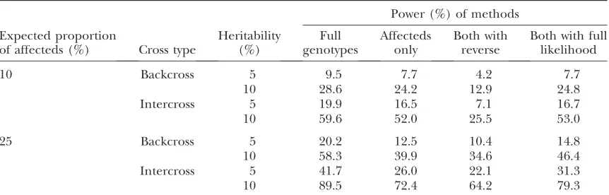
Power for all combinations of parameters based on 10,000 simulation replicates is shown in Table 3. For each of the scenarios considered, the highest power was obtained by full genotyping with standard analysis. Affecteds only analysis and constrained full-likelihood analysis with partial genotyping had comparable power to detect a QTL, with slightly lower power in the affecteds only analysis under all investigated scenarios. Finally, reverse analysis with partial genotyping showed notably lower power to detect a QTL compared to the other three approaches.
When the affected phenotype is rare, an affecteds only analysis can provide power comparable to anal-ysis of the full cross and requires only a small fraction of the genotyping. To check for spurious evidence due to segregation distortion, further genotyping of un-affecteds can serve as a useful supplement to un-affecteds only analysis, particularly when incorporated by con-strained full-likelihood analysis, and with greater im-provements seen when the affected phenotype is more common. Although analysis of affecteds and unaffec-teds using the reverse approach, LODR, has lower power than other approaches, we should keep in mind that this approach is more robust to segregation dis-tortion than the constrained full-likelihood analysis, which can suffer from reduced power in the presence of segregation distortion. The relatively weaker perfor-mance of the reverse approach, LODR, suggests this robust strategy is more suitable as a follow-up check for segregation distortion, rather than as a genomewide QTL mapping strategy.
DISCUSSION
genotyp-ing. As alternatives to standard interval mapping, we presented a reverse approach of modeling genotypes conditional on phenotypes and also a full-likelihood approach. Our suggested modifications to the standard approach of Xuand Atchley(1996) are developed in
terms of fundamental likelihood modeling strategies. Accordingly, a key contribution here is our presentation of approaches to binary trait analysis using a cohesive likelihood framework, elucidating fundamental rela-tionships among the methods. Our formal develop-ment of allele sharing methods presented as the reverse approach, LODR, led to the use of hidden Markov models to allow interval mapping in the reverse and full-likelihood approaches (appendixes aandc). Through
analytical comparisons, we found that our reverse approach, LODR, is identical to a full-likelihood ap-proach at both marker and nonmarker locations.
We also proposed another version of the reverse approach, LODR,seg, which incorporates a segregation assumption of the expected genotype proportions based on the type of cross that was performed. This approach formalizes a natural method of analysis for dealing with genotypes on affecteds only and presents it in a more general form that can be applied with genotypes on both affecteds and unaffecteds. We found the log10 -likelihood ratio, LODR,seg, could be decomposed as the sum of two types of evidence: (1) deviation of genotype proportions by phenotype group and (2) segregation distortion. For the case of genotypes on affecteds only, incorporating the segregation assumption was espe-cially crucial, as it provided a view of evidence for a QTL where none was available by LODRor LODF.
The inclusion of evidence for segregation distortion was deemed inappropriate in dealing with data having genotypes available on both affecteds and unaffecteds. For this case, we proposed incorporating the segrega-tion assumpsegrega-tion using a constrained full-likelihood
approach. In this way, the segregation assumption was imposed under both the null and alternative hypothe-ses, so that the resulting test statistic, LODN
Full;seg, did not contain evidence for segregation distortion. Eliminat-ing evidence for segregation distortion helps ensure that a large LOD score indicates evidence of a QTL, as segregation distortion can arise simply by random chance, systematically as a result of genotyping error, or as a result of embryonic lethal alleles that are unrelated to the trait of interest.
An understanding of these approaches as they relate to one another helps us to decide which method to use on the basis of the existing pattern of selective genotyping. In the case that we have genotyped every-body in our sample, we are not interested in overall evidence for segregation distortion and would choose a standard approach LODF. On the other hand, if we have genotyped affecteds only, the standard approach does not allow us to detect association. In this case, all evidence of association will be captured as evidence for segregation distortion, which shows up only with use of LODR,segas LODseg.dist..
Since full genotyping of a cross can be costly, while affecteds only analysis can be prone to spurious evi-dence, a reasonable balance is to genotype some affecteds and some unaffecteds. Specifically, we recom-mend an initial screen with genotypes on all affected individuals and an equal number of unaffecteds, fol-lowed by analysis of the full cross in genomic regions of interest. As demonstrated in the application, this
economical strategy can be an effective way to charac-terize QTL from the full cross and requires only a fraction of the genotyping. The ideal selective genotyp-ing approach for any particular study may of course vary from this recommendation and could be studied as a function of animal rearing and phenotyping costs relative to genotyping cost.
TABLE 3
Power to detect QTL using four different strategies for binary trait mapping
Power (%) of methods Expected proportion
of affecteds (%) Cross type
Heritability (%)
Full genotypes
Affecteds only
Both with reverse
Both with full likelihood
10 Backcross 5 9.5 7.7 4.2 7.7
10 28.6 24.2 12.9 24.8
Intercross 5 19.9 16.5 7.1 16.7
10 59.6 52.0 25.5 53.0
25 Backcross 5 20.2 12.5 10.4 14.8
10 58.3 39.9 34.6 46.4
Intercross 5 41.7 26.0 22.1 31.3
10 89.5 72.4 64.2 79.3
The reverse approach, LODR, with no segregation assumption is a natural method of analysis for data with genotypes on affecteds and some unaffecteds. Although this approach was shown to be quite similar to the standard approach LODFat marker locations, we prefer LODRas it is not susceptible to biased parameter estimates and so produces more reliable results in between markers.
A full-likelihood analysis with constrained maximiza-tion under both the null and alternative hypotheses, presented as LODN
Full;seg, is another reasonable way to approach selective genotyping data with both affecteds and unaffecteds. Incorporating the segregation assump-tion in this setting is a practical compromise to preserve the evidence reported in an affecteds only analysis while bringing in unaffected individuals. The drawback, as seen in the Listeria example (Boyartchuket al.2001),
is that evidence can be attenuated when there is overall segregation distortion in the data. Still, our computer simulation studies indicate constrained full-likelihood analysis offers notably higher power than the reverse approach, LODR, across a variety of parameter val-ues. Thus, our power studies suggest constrained full-likelihood analysis is preferable as long as there is no pervasive segregation distortion in the cross.
A further limitation of the reverse approach lies in the treatment of multiple-QTL models. While single-QTL models may be set up quite naturally by conditioning genotypes at a single locus on the observed phenotypes, modeling genotypes at multiple loci can be much more cumbersome. Instead, when exploring multiple-QTL models with data on both affecteds and unaffecteds available, the standard approach of conditioning phe-notypes on gephe-notypes is more natural. The close re-lationship between the forward and reverse approaches in a single-QTL scan makes it quite reasonable to go ahead with the forward approach for the consideration of multiple-QTL models in the presence of selective genotyping. When using the forward approach for multiple-QTL mapping under selective genotyping, inferences at nonmarker positions may still be some-what unreliable, while entirely valid results will be produced for models involving marker positions only.
After performing an analysis of a cross experiment under selective genotyping, we may always follow up by genotyping all individuals in genomic regions of interest identified from the initial scan. Such follow-up will be especially important if the initial scan is performed with affecteds only, since this strategy is most sensitive to spurious evidence due to segregation distortion.
We thank William Pu at the Children’s Hospital in Boston for presenting us with data motivating this research. This work was supported in part by National Institutes of Health grant GM074244 (to K.W.B.) and by a National Science Foundation Graduate Research Fellowship (to A.M.).
LITERATURE CITED
Boyartchuk, V. L., K. W. Broman, R. E. Mosher, S. E. D’Orazio, M. N. Starnbach et al., 2001 Multigenic control ofListeria
monocytogenessusceptibility in mice. Nat. Genet.27:259–260. Broman, K. W., 2003 Mapping quantitative trait loci in the case
of a spike in the phenotype distribution. Genetics163:1169– 1175.
Broman, K. W., H. Wu, S. Senand G. A. Churchill, 2003 R/qtl: QTL mapping in experimental crosses. Bioinformatics 19: 889–890.
Chen, Z., and J. Liu, 2009 Mixture generalized linear models for multiple interval mapping of quantitative trait loci in experimen-tal crosses. Biometrics (in press).
Churchill, G. A., and R. W. Doerge, 1994 Empirical threshold val-ues for quantitative trait mapping. Genetics138:963–971. Coffman, C. J., R. W. Doerge, K. L. Simonsen, K. M. Nichols, C. K.
Duarteet al., 2005 Model selection in binary trait locus map-ping. Genetics170:1281–1297.
Dempster, A., N. Lairdand D. Rubin, 1977 Maximum likelihood from incomplete data via the EM algorithm (with discussion). J. R. Stat. Soc. Ser. B39:1–38.
Deng, W., H. Chenand Z. Li, 2006 A logistic regression mixture model for interval mapping of genetic trait loci affecting binary phenotypes. Genetics172:1349–1358.
Faris, J. D., B. Laddomadaand B. S. Gill, 1998 Molecular mapping of segregation distortion loci inAegilops tauschii.Genetics149: 319–327.
Hauser, E. R., and M. Boehnke, 1998 Genetic linkage analysis of complex genetic traits by using affected sibling pairs. Biometrics 54:1238–1246.
Henshall, J. M., and M. E. Goddard, 1999 Multiple-trait mapping of quantitative trait loci after selective genotyping using logistic regression. Genetics151:885–894.
Holmans, P., 1993 Asymptotic properties of affected-sib-pair link-age analysis. Am. J. Hum. Genet.52:362–374.
Huang, H., C. D. Eversley, D. W. Threadgill and F. Zou, 2007 Bayesian multiple quantitative trait loci mapping for com-plex traits using markers of the entire genome. Genetics176: 2529–2540.
Lambrides, C. J., I. D. Godwin, R. J. Lawn and B. C. Imrie, 2004 Segregation distortion for seed testa color in Mungbean (Vigna radiataL. Wilcek). J. Hered.95:532–535.
Lander, E. S., and D. Botstein, 1989 Mapping Mendelian factors underlying quantitative traits using RFLP linkage maps. Genetics 121:185–199.
Lander, E. S., P. Green, J. Abrahamson, A. Barlow, M. J. Daly
et al., 1987 MAPMAKER: an interactive computer package for constructing primary genetic linkage maps of experimental and natural populations. Genomics1:174–181.
MacCluer, J., J. Vandeburg, B. Readand O. Ryder, 1986 Pedigree analysis by computer simulation. Zoo Biol.5:149–160. McIntyre, L. M., C. J. Coffmanand R. W. Doerge, 2001
Detec-tion and localizaDetec-tion of a single binary trait locus in experimental populations. Genet. Res.78:79–92.
Moran, J. L., A. D. Bolton, P. V. Tran, A. Brown, N. D. Dwyer
et al., 2006 Utilization of a whole genome SNP panel for effi-cient genetic mapping in the mouse. Genome Res.16:436–440. Nelder, J., and R. Mead, 1965 A simplex method for function
min-imization. Comput. J.7:308–313.
Risch, N., 1990 Linkage strategies for genetically complex traits. II. The power of affected relative pairs. Am. J. Hum. Genet.46:229– 241.
Xu, S., and W. R. Atchley, 1996 Mapping quantitative trait loci for complex binary diseases using line crosses. Genetics143:1417– 1424.
Yi, N., and S. Xu, 2000 Bayesian mapping of quantitative trait loci for complex binary traits. Genetics155:1391–1403.
APPENDIX A: THE REVERSE APPROACH AT NONMARKER LOCATIONS
We describe the algorithm for obtaining ˆfhere. Analogous methods for obtaining ˆfDand ˆfD˜ follow directly by
applying the same algorithm within each of the two phenotype groups.
Given the full set of observed genotype data Oi ¼ (O1i,. . ., Opi) for a single individual at the p putative
QTL positions to be considered, letGi denote the underlying genotype at the mth putative site of interest. We
can expand the probability of the observed marker data given the underlying genotype at the putative QTL of interest as
qig¼PrðO1i;. . .;Oðm1ÞijGi¼gÞ3PrðOmijGi ¼gÞ3PrðOðm11Þi;. . .;OmijGi¼gÞ
¼bl
miðgÞ3eðg; OmiÞ3brmiðgÞ;
where the conditional probabilities of observed marker data,bl
mi(g) andb
r
mi(g), to the left and right of putative QTL
may be obtained inductively using the backward equations in the context of hidden Markov models (HMMs) (Lander
et al.1987). Here,e(g, Omi) is the corresponding emission probability at the mth genetic position of interest for
individuali, which can also be interpreted as the genotyping error rate.
The likelihood function for the parameterfbased on the observed genotype dataOion individualsi2{1,. . .,nobs} is
likðfÞ ¼Y
nobs
i¼1
PrðOi;fÞ
¼Y
nobs
i¼1
X
g2fAA;ABg
½qigPrðGi¼g;fÞ:
At iteration s 1 1, we have the parameter estimate, ˆfðsÞ. In the E-step, we calculate the expected number of individuals with genotypeAAat the putative QTL of interest as
ˆ nðAAs11Þ¼
Xnobs
i¼1
PrðGi¼AA;Oi;fˆ ðsÞ
Þ
PrðOi;fˆ ðsÞ
Þ
¼X
nobs
i¼1
ˆ
fðsÞqi;AA
ˆ
fðsÞqi;AA1ð1fˆ ðsÞ Þ qi;AB
: ðA1Þ
In the M-step, the updated parameter estimate is simply ˆfðs11Þ¼nˆAAðs11Þ=nobs. A reasonable initial estimate offis the
sample average of conditional genotype probabilities, ˆfð0Þ¼ ð1=nobsÞPnobs i¼1pi;AA.
APPENDIX B: ALTERNATE REPRESENTATIONS OF THE FULL LIKELIHOOD We may expand our presentation of the full likelihood from Equation 1 as follows:
likðfD;fD˜;pÞ ¼
YN
i¼1
PrðDi;Oi;fD;fD˜;pÞ
¼ Y
nobs
i¼1
PrðOijDi;fD;fD˜Þ
Y
N
i¼1
PrðDi;pÞ
ðB1Þ
¼likðfD;fD˜jDÞ likðpÞ: ðB2Þ
Here, the pattern of missing genotypes generated by selective genotyping depends only on the observed phenotypes, D, and is conditionally independent of the underlying genotypes,G, givenD. Hence, the model implicitly condi-tions on the pattern of selective genotyping, with PrðOi jDi;fD;fD˜Þ ¼1 for all ungenotyped individuals,
i2 fnobs11;. . .;Ng.
likðpAA;pAB;fÞ ¼Y
N
i¼1
PrðDi;Oi;pAA;pAB;fÞ
¼Y
N
i¼1
PrðDijOi;pAA;pABÞ PrðOi;fÞ; ðB3Þ
where ungenotyped individuals,i¼nobs11,. . .,N, are incorporated by applying the marginal genotype probabilities as mixing proportions in modeling disease status using a binomial model withp¼pAAf1pAB(1f). To find the
appropriate MLEs, note that the likelihood in (B3) is a reparameterization of (B1). Specifically, the parameters of interestpAA,pAB, andfcan be written in terms offD,fD˜, andp:
f¼fDp1fD˜ ð1pÞ
pAA¼fDp
f
pAB¼ð1fDÞ p
1f : ðB4Þ
Then, the appropriate MLEs forpAA,pAB, andfin (B3) can be obtained as plug-in estimates using the relationships in (B4). We have provided these MLEs for completeness, but if our primary aim is the appropriate likelihood-ratio statistic, then calculating these MLEs is unnecessary.
APPENDIX C: CONSTRAINED FULL-LIKELIHOOD ANALYSIS AT NONMARKER LOCATIONS
To start, we incorporate the constraint by transforming the expression in (2) to yieldfD˜ ¼ ðffDpÞ=ð1pÞ.
Hence, our constrained likelihood is equivalent to a two-parameter model in which each individual has the following contribution to the likelihood,
likðfD;p;Oi;DiÞ ¼PrðOijDi;fD;pÞ PrðDi;pÞ;
with observed genotypes modeled according to disease status as
PrðOijDi;fD;pÞ ¼
P
g2fAA;ABgPrðGi¼g;fDÞ qig; Di¼1 P
g2fAA;ABgPrðGi¼g;fD˜ ¼
ffDp
1p Þ qig; Di¼0
(
ðC1Þ
for genotyped individuals and identically equal to one for ungenotyped individuals.
At iterations11, we have the parameter estimate, ˆfðDsÞ. In the E-step, we calculate the expected number of affected and unaffected individuals with genotypeAAat the putative QTL as shown in (A1).
In the M-step, the updated parameter estimates are obtained by maximizing the likelihood function in (C1), using a numerical optimization approach such as that of Nelder and Mead (1965). Similar to the EM for the reverse
approach above, we use the sample average of conditional genotype probabilities,pig, among diseased individuals as an
initial guess forfDand take the sample averagenD=N as the initial estimate forp.
APPENDIX D: MORE RELATIONSHIPS BETWEEN THE FULL AND REVERSE APPROACHES
Full likelihood vs. reverse approach: Let LODnobs
Full be the LOD score based on full likelihood for genotyped individuals i ¼1,. . ., nobs only and LODNFull be the LOD score from full-likelihood analysis using all individuals i¼1,. . .,N, whether genotyped or not. We see the following analytic results comparing LODnobs
Fullto LODRfrom the reverse approach:
LODnobs
Full¼log10
PrðOjD;fˆD;fˆD˜Þ PrðD;pˆÞ
PrðO;fˆÞ PrðD;pˆÞ
¼log10 PrðOjD;fˆD;fˆD˜Þ PrðO;fˆÞ
¼LODR:
Likewise, we can compare LODN
with the conditional multipoint marker probabilities identically equal to one for all ungenotyped individuals. Using Equation B2 above, we see that
LODNFull¼log10 maxfD;fD˜
Qnobs
i¼1PrðOijDi;fD;fD˜Þ
maxf
Qnobs
i¼1PrðOi;fÞ
3 maxp
QN
i¼1PrðDi;pÞ
maxp
QN
i¼1PrðDi;pÞ
¼log10 PrðOjD;fˆD;fˆD˜Þ PrðO;fˆÞ
¼LODR;
where the estimated parameters ˆfDand ˆfD˜ are the MLEs specified in themethodssection.
Constrained full likelihoodvs.modified reverse approach:It is difficult to work with the constrained full likelihood analytically. However, we can derive the following inequality to put an upper bound on LODN
Full;seg. First note that constrained likelihood must be bounded above by the unconstrained likelihood so
max fD;fD˜;pjf¼1=2
likðfD;fD˜;pÞ# max
fD;fD˜;p
likðfD;fD˜;pÞ
¼likðfˆD;fˆD˜Þ likðpˆÞ;
where ˆfD, ˆfD˜, and ˆpare the unconstrained MLEs.
Plugging into LODN
Full;seg, we find
LODNFull;seg¼log10
maxfD;fD˜;pjf¼1=2likðfD;fD˜;pÞ
maxplikðf¼1=2;pÞ
#log10 likðfˆD;fˆD˜Þ likðpˆÞ likðf¼1=2Þ likðpˆÞ
¼LODR;seg: