42
Composite Sketch Based Face Recognition
Using ANN Classification
Shivaleela Patil, Dr.Shibhangi D C
Abstract: Today Computer based Technologies have been boosted much procedure and process involved in preparations of crime view documents. In this view point, photography is the first step and important clue to start or to solve investigation of crime, helps in tracing and matching the facial composites against database related to the memory of eyewitness. The facial composites i.e., sketches drawn by the artists or software aids the law enforcement using the description given by the witness in direct to depict the suspects and missing persons, which are posted on public places and helps in recognizing. These methods are found to be useful and many criminals have been recognized through this way. Since the combined sketches provide better and accurate and 80% of law enforcement insists for composite sketches rather than forensic sketch. Therefore in this proposed system, we are focusing on composite sketch based face recognition. First detect the face section using AdaBoost algorithm and detect the facial mechanism using the geometrical model of the face. Features are removed from each individual facial parts by using multi-scale local binary patterns (MLBP) and Tchebichef moment invariant feature. Finally, the ANN classifier is trained to identify the person classified.
Index Terms: Forensic Sketch, Composite Sketch, Facial Components, Geometrical Model, Multi-Scale Local Binary Patterns (MLBP), Tchebichef Moment Invariant feature and ANN Classifier.
—————————— ——————————
1.
INTRODUCTION
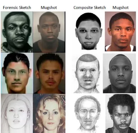
In computer vision face detection is an important application for human face detection or authentication of human being. 9/11 tragedy in India after the incidence, Need improvement of technology for identification of the suspect and recognition has been improved from last 20 year, studying a identification of human face but structure computational model for identification still difficult task. Today identification of human face has improved in field of multimedia, as face plays a major role in recognition of people with respect to one another and also in variety of application such as security system, credit card verification, illegal recognition and a lot of application is used. Face identification is one of the important applications for assistance in law enforcement. If the victims fingerprint or images captured in the surveillance camera are found during criminal investigation, they act as clue to recognize the victims using biometric technique. In the cases if the crime present with the absence of above data, police team looks for eyewitness and forensic artist to work with proof to draw a sketch of the criminal. Sketches drawn based on such condition can be of two type‘s called forensic sketch or composite sketch. Forensic sketch artist are used to draw the sketch by description provided by the witness known as forensic sketch and by using composite software tools facial composite are drawn for the suspect face. Once the sketch is ready it is send to law enforcement officers and for social Medias with the hope to find the suspect. Composite sketches are most generally used to recognize the victims, where as a forensic sketch required well trained artist for drawing and sculpting. In composite sketches there exist many software devices tools, which are even used by the non artist to sketch. As per the review given in [03] 80% of law enforcement uses composite sketches. It has become a famous substitute for illegal justice and other agency of law enforcement. Small number of extensively used software kits to produced computerized sketches contains Photo-Fit, IdentiKit, Mac-a-Mug, FACES and EvoFIT. This software permit a synthesizing sketches by selecting a sketch by choosing a set of facial component, examples eye, hair, eyebrow, mouth, shape, nose and eyeglass. Figure 1 shows the difference between forensic sketch and the composite sketch.
Figure 1: Difference between Composite Sketches and Forensic Sketches
43
robot vision, compression data and visual pattern recognition. Techniques of moment invariants have been confirmed to be a device for application of pattern recognition, Due to their sensitivity to the description of object features. One more texture feature approach called LBP is a nonparametric approach proposed for texture analysis and has proved to be a simple yet powerful approach to describe local structures by briefing the local structures of an input picture by examining every pixel with its nearest pixels. LBP has been testing with facial representation in many applications like face detection, face identification, facial expression analysis, age classification and other related applications. In the proposed system we analyze an identification procedure for recognizing the composite sketch with the database. As the initial step, we locate the face region from the input image. As the next step different facial component likes mouth, nose, and eyes are detected by examining the relative relationship and distance between the components by referring the geometrical model of the face structure. By cropping separated components, Tchebichef moment and MLBP feature are extracted and trained to the ANN classifier to create a knowledge base. Finally query image is matched with the created knowledgebase to classify by recognizing the person.
2
LITERATURE
SURVEY
Shubhangi et al. [01] have developed a procedure to compare composite and photograph in the mug shot database known for component-based representation. Primarily they have renormalized mugshot database related to geometric transformation, colour space conversion and image enhancement. Later facial components localization is applied Active Shape Model (ASM) and Viola-Jones algorithm. As the next step for every component, matrix renormalizes cross-correlation and the nearest neighbor feature is extracted. For every device same measurement, normalization of score and fusion are performed between the composite sketch and database. Archana Uphade et al. [02] had used publically obtainable software to produce composite sketches they have followed CBR procedure to recognize the sketch with mug shot database. By using active shape model landmarks the face are recognized. As per their method, instead of comparing the whole image with the database, only face components are trained in the knowledgebase. When the query image is compared with the knowledgebase, only facial components are extracted using ASM model to measure the similarity score. To match the query image with the photos, Canny Edge Detection and K-Means Algorithms are employed.
Deepinder Singh et al. [03] had utilized
geometric features of the face such as eyes,
eyebrows, lips, and nose, shape of the face and
their measured length and ratios of width. Five
different
modules
proposed
are:
Facial
component extraction, measure of ratios of
Width, Length and Area. Each component is
signified in a vector form. They have computed
zero-mean vector by finding the mean of each
vector and subtract it from each component to
get the zero-mean set of vectors. Finally, search
for query sketch image with the knowledgebase
is done.
44
mechanism of composite sketches, but it is seen that achieving good accuracy is still a challenging task. Hence to improve the accuracy of the system, an efficient approach is proposed. Proposed system is explained in detail below.
3. METHODOLOGY
The architecture of the proposed methodology is as depicted in Figure 2. The computer generated composite sketches are considered as the input images for further processing. The proposed composite sketch based face detection system includes two process training and testing process. In training process database images are trained, each image face region is located, pre-processed and texture features like Multi-Scale Local Binary Pattern (MLBP) and Tchebichef moment invariant feature are extracted and the resulted feature vector are stored in the database for matching with test images. Next part is testing process, build up with five different modules namely pre-processing Module where input images are resized and conversion from RGB to gray scale image is performed [09]. In Face detection module the location of face region is located and cropped. For the identification of the face, different facial components of the face are located referring the geometrical structure of the face. As the next module each extracted facial components like eyes, nose and mouth features are extracted using Multi-Scale Local Binary Pattern (MLBP) and Tchebichef moment invariant features techniques. Finally, extracted feature of a particular person needs to be identified, for this an Artificial Neural Network (ANN) classifier is trained. Here the classifier is initially trained with composite sketches features taken from the database in the training phase to create a knowledgebase. Every time a test feature is extracted they are compared with the knowledgebase using ANN classifier to get the classified output.
Pre-processing Facial Component
Extraction Feature Extraction ANN Training
Query Image Pre-processing Feature Extraction ANN Classification
· RGB to Gray Conversion
· Resizing
· Geometrical Model
Knowledge Base Testing
Facial Component Extraction Training
Recognized Person Face Detection
Face Detection
· MLBP
· Tchebichef Moments
Composite Sketch Composite Sketch
Figure 2: Architecture of the Proposed System.
3.1 Pre-Processing
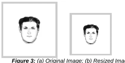
Pre-Processing is a lower level process performed on images. These approach asses in improving the data exist in the image by filtering the distortions or enhance the relevant information for further analysis. Image resize and RGB to gray color conversion are the step of preprocessing step. The main purpose of resizing the input picture is to decrease the amount of pixel value so that operations become faster and values passed to ANN will be limited. Image resizing to obtain proper resolution and measurement is important as over-size or resize image may lead to information loss. If we select the image to a smaller resize value than data of ANN and the database will increase, resulting in decreasing the processing speed of the system. The composite sketches present in the database have been standardized to 200 pixels in length and
150 pixels in width. Figure 3: (a) Shows the Original Image and (b) shows the image resized to 200x150.
(a) (b)
Figure 3: (a) Original Image; (b) Resized Image
The second step we have employed is grayscale computation, where image transforms from the RGB (3D) domain to grayscale 2D domain. The reason to perform this task is to reduce the difficulty in performing the operations with respect to each color domain independently and then transforming images to grayscale. Working with lighter intensities instead of color intensities reduces the problem. Along with that grayscale images are store in memory space.
3.2FACE DETECTION
Face detection technique is based Viola and Jones algorithm, which guide the classifier by a different set of patterns with face and nonface images. A common effort is to operate a wide number of training examples and hence solve the problem of classification accurately. Using face detection technique, identification of face will be done as the initial step.
In the Adaboost algorithm initially Training set say will be the input, belongs to a domain or instance space , and label denotes finite label space . Here we are focusing on binary case where
At each turn, AdaBoost make a call to a weak or base learning algorithm which consider a sequence of training as input for examples and also the distribution or a set of defined weights for each training examples, For an input the weak learner calculates a weak classifier , Where will be in the form of . We interpret the sign of ) as the predicted label to be assigned to instance x. Once the weak classifier has been received, AdaBoost chooses a parameter that intuitively measures the importance that it assigns to as in Algorithm 1. The idea of boosting is to use the weak learner to form a highly accurate prediction rule by calling the weak learner repeatedly on different distributions over the training examples. Initially, all weights are set equally, but each round the weights of incorrectly classified examples are increased so that those observations that the previously classifier poorly predicts receive greater weight on the next iteration [10].
Algorithm 1: AdaBoost
Input: ( where
Initialize: weights Iterate
1.
instruct weak learner utilizing distribution2.
Get weak classifier3.
Choose45
5.
where is a normalisation factorOutput: the final classifier output as shown in Figure 4(a) and (b).
(a) (b)
Figure 4: (a)Preprocessed Image (b) Clasifier Output Image
3.3 FACIAL COMPONENT EXTRACTION
Measuring geometric of face regions [13] such as eye, nose and mouth, the facial feature extracting commonly refers to the identification of eye, nose, eyebrows, lips, and different significant parameters of the face. Identification of image region in face image/sketches will use geometric feature method. In this method, the facial feature is extracted using relative location and size of the face.
3.1.1 Extraction Methodology
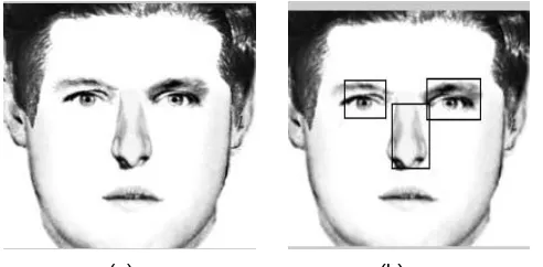
In the proposed work [12], to recognize a composite sketch, extraction of the facial component is required from images. Geometric feature method is used to predicate the different facial component. Using one algorithm it is not possible to extract the entire facial components. In the facial component recognition most significant step to track eye position, the rule of prediction of the different facial component is implemented to the row on which there is an existing of eyeball. Here we have used Geometric model as shown in Figure 5. To get the positions in the facial component, applicability of proper algorithms is very necessary as depicted below.
a) Eye Region Extraction [05]
After the face detection, we first guess the expected region of an eye using facial geometry. The eye is located in the upper part of the face in frontage face image.
Step.1: Image is converted into binary form
Step.2: Perform open and close operations
The opening operation smoothes the contour of the skin region, breaks narrow isthmuses, and eliminates small islands and sharp peaks or capes. The closing operation fuses narrow breaks and long, thin gulfs; eliminates small holes, and fills gaps on the contours. A rectangular structuring element is used in the opening and closing area.
Step.3: By applying the region props, the biggest binary object obtained in the upper left quarter region is identified as left eye region and marked with a bounding box. Similarly, right eye region is
identified and marked with a bounding box as shown in Figure 5 (a) and (b).
(a) (b) (c) (d) (e)
(f) (b)
Figure 5: (a) Original Image; (b) Marked with Bounding Box Image
b) Nose Region Extraction
Step.1: Achieve the bounding box coordinates of
left eye region.
Step.2: By investigating the nose region we put in up constant values to set a new ordinary set of co-ordinate and deduct the width by a constant value as shown in the Equation (2), (3), (4) and (5).
A Bounding box is distinct with the new set of coordinate values as shows in Figure 6 (a) and (b).
(a) (b) (c) (d) (e) (f)
(g) (b)
Figure 6: (a) Preprocessed Image; (b) Marked with Bounding Box Image
c) Mouth Region Extraction
Step.1: To get the harmonize values from the bounding box of nose region, by adding up the constant value to the height of the nose, x- coordinate and y- coordinate value can be predicted using Equation (6) and (7).
46
(a) (b) (c) (d) (e) (f)
(g) (b)
Figure 7: (a)Preprocessed Image; (b)Marked with Bounding Box Image
3.4 MULTI-SCALE LOCAL BINARY PATTERNS
The appearance, structure and arrangement of the part of an object within the image refer to the texture of the image [15]. The LBP operator, start by Ojala et al [06] has been a dominant measure of picture texture. Local Binary Patterns (LBP) is a non-parametric texture patterns descriptor. Texture patterns from a 3x3 neighborhood of an image patch as shown in Figure 8 which encode the basic LBP operator. The threshold is to be considered as center pixel. Each neighboring pixel is compared next to the center pixel to produce an 8-bit binary string. At last, binary string converted into decimal label according to assigned weights. The amounts of different local patterns are composed into a histogram that is used as a texture descriptor as defined in Equation (10).
Where, is the gray value of the centre
point , is the number of
neighborhood point on a circle of radius with , as the centre.
Threshold on center value
“00111110” Binary LBP Code
100 126 124
200 165 205
212 190 195
0 0 0
165
1 1
1 1 1
1
0 256 128
2 64
4 16 32
3X3 neighborhood 3x3 binary pattern
weights
Figure 8: Calculation of a Basic LBP
The LBP operator has been effectively utilized in the image identification for good robustness on the influence of
illumination, angle, and occlusion. However, it does not achieve good when happened to face several illumination changes and it is too blurred to describe the unique details contained in an image. Thus, an improved multi-scale LBP operator (MLBP) is implemented to extract more distinctive data and improve recognition achievement. Comparison for center point with multiple neighborhood points of different radii and same radial direction with each other is done.
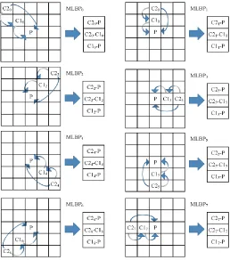
Figure 9: Structure of the MLBP Operator
In this article, two radii and eight radial directions are
chosen, which are similar to two LBP operators of different radii. The structure of the MLBP operator is shown in Figure 9. An area of 5 × 5 points is chosen, which is collected of two squares with different radii, but centered its neighborhood point on the inner square with the smaller in the similar point P. is the area point on the inward square with the smaller radius and is the neighborhood point on the external square with the greater span . The pixel value of eight radial directions is contrasted with each other as per the thick arrows signs. The 3 × 8 local difference values of three arrows in eight clockwise orientations from the canter point compose the whole MLBP operator. Referring to the definition of the original LBP operator just the imperative sign data is coded by in Equation 11;
Where , is the
47
descriptors into the MLBP features, more comprehensive and distinguishable texture information can be obtained than using only one of them. Besides, the radii R1, R2 are changeable to obtain better performance [20].
3.4.1 Moment Invariant
Moment functions with discrete orthogonal kernel are implemented basically with the aim of deriving enhanced feature representation capability pattern analysis applications. Discrete orthogonal moments are less susceptible to noise and numerical instabilities when compared with geometric and other types of non-orthogonal moments. Tchebichef polynomials have the advantage of being orthogonal functions of unit weight over an integral domain and having a simple recurrence formula for polynomial computation, DTM is computed by projecting the Pre-processed image onto a set of Tchebichef polynomial kernels, which include basis functions of the DCT as a special case. The
moment of
order is obtained from the Tchebichef kernel .The orthogonality between Tchebichef polynomials ensures exact image reconstruction from the set of moments . The value of can be interpreted as the connection between's the picture and the discrete Tchebichef polynomial . These bit capacities are described by a wavering conduct, demonstrating a sine-like profile. Figure 10 (a) and (b) demonstrates the arrangement of Tchebichef portions for in both spatial and recurrence spaces. As seen as the request of the bit builds the vitality of a part work as a tendency to be moved in higher frequencies [11].
Figure 10: (a) Tchebichef Kernels Spatial Domains; (b) Frequency Domains
The kernel acts as a filter for the calculation of . The extent of will be higher for images oscillating at a comparative rate to along the two direction [12]. It is a fascinating property for surface examination since surface includes the spatial reiteration of force designs. Consequently, a depiction of surface assets can be obtained by estimating the reliance existing apart from everything else size on the request s, which is identified with the recurrence substance of pieces. For this reason, the accompanying component vector
is proposed defined as Equation (12):
The element gives data about the properties of a texture and can be seen as a face mark. To assess the particular characteristics caught by ), the conduct of Tchebichef pieces in both spatial and frequency domains is studied.
Start
Get the Size of Image
Calculate the Moment Order(p,q)
Calculate Tchebichef Polynomials using Recurrance Relations
Calculate Tchebichef Moments
Stop
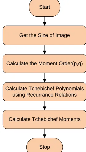
Figure 11: Flow Chart of Tchebichef Polynomial
Tchebichef polynomials ( ) are the least complex among discrete orthogonal elements of unit weight, and in this way, a big number of the diagnostic assets of the ordinary minutes can be effectively determined and contrasted. The discrete ‘s are characterized as in Equation 13.
‗s have mathematical relations including real coefficients which make them reasonable for characterizing change for picture pressure and recreation. For a given positive number and esteem in the range by utilizing the scale factor the scaled Tchebichef polynomial [19] is given as in Figure 11,
3.5ARTIFICIAL NEURAL NETWORKS
48
biological neurons. Some of the major attributes of ANN such as they can learn from examples, generalize well on unseen data and able to deal with a situation where the input data are incomplete or fuzzy. There have been hundreds of different models considered as ANNs since the first neural model been introduced by McCulloch and Pitts that includes General Regression Neural Network, which will be briefly discussed in the next section. The differences in those models might be the functions, the accepted value, the topology and learning algorithm. There are also many hybrid models where each neuron has more properties. Neural networks can recognize patterns, even when the information consist of these patterns is noisy or incomplete. Previous works show that neural networks are very good pattern recognizers since they can learn and build unique structures for a particular problem [14]. The total features extracted from each samples is 59. The total training classes taken in the proposed work is 10. Training involves feeding the training samples as input vectors through a neural network, error calculation of the output layer and weight adjustment to minimize error in the network. In the research work we are making use of 170 neurons at input layer, 45 neurons at hidden layer and 10 neurons at output layer. The learning rate chosen is = 0.9, momentum term = 0.6, show = 50 and epochs = 100. Once the network is ready to be trained, the samples are automatically divided into training, validation and test sets. The training set is used to teach the network. Training continues as long as the network continues improving on the validation set. The test set provides a completely independent measure of network accuracy.
4
EXPERIMENTAL
RESULTS
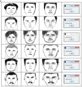
The PRIP Viewed Software-Generated Composite (PRIP-VSGC) [21]database used in the paper contains 123 composites generated using FACES [22] and using Identi-Kit [23]. Figure 12 shows a result for all the intermediate results obtained taking composite sketch as the input from the dataset taking 120 composite sketches. Figure 12:(a) depicts the Input image, (b) is the Face detected, (c) is obtained after cropping the face area; (d) shows the cropped Left eye region; (e) shows the cropped Right eye region, (f) shows the cropped Nose region, (g) shows the cropped Mouth region; (h) shows the Facial Component Identification result. From these dataset, results for only three sketches are shown in Figure 13. Figure 13(a) shows the pre-processed images or sketches of the original images considered from the set of the dataset. Figure 13(b) represents the face area detection of the input by using AdaBoost Algorithm and geometric measurements of facial components are extracted by using Multi-scale LBP operator (MLBP) and Techbichef moment as shown in Figure 13(c). ANN Classifier is trained to match the sketches with the dataset and resultant is shown in Figure 13(d). The classifier gives the respective class as the matched output out of trained 10 classes. The confusion matrix is a prediction analysis which is used to calculate true positive, true negative, false positive and false negative rates as in Table 1. It helps to analyze the performance of the methodology. By using confusion matrix, we can calculate accuracy, precision sensitivity and recall parameters as in Equation (15), (16), (17).
The amount of precision of a quantity is called as accuracy which is given by the formula,
Precision is nothing but scientific or mechanical exactness which is given by,
Sensitivity, True positive rate and Recall rate is given by,
Sensitivity is a degree of responsiveness or awareness to external or internal changes.
(a) (b) (c)
(d) (e) (f)
(g) (h)
49 Figure 13: (a) Composite Sketch Input Image; (b) Face
detection; (c) Facial Component Identification; (d) classified output.
Figure 14: Accuracy Graph for the Proposed and the Existing System
5.
CONCLUSION
50
classification systems can prove extremely useful for quick and efficient classification of face. The accuracy of the current proposed approach is comparable to those reported in contemporary works. The experimental results explained that the proposed method is effective. Experiments are conducted on 120 composite images of PRIP Viewed Software-Generated Composite (PRIP-VSGC) database. The model used multiple feature extraction methods to reduce the complexities and computational time. In order to increase classification performance ANN classifier is used. The proposed algorithm is evaluated on PRIP-VSGC dataset resulting in accuracy of 95%.