The Maximum Lq-Likelihood Method: an Application to Extreme Quantile Estimation in Finance

RECent: c/o Dipartimento di Economia Politica, Viale Berengario 51, I-41100 Modena, ITALY

WORKING PAPER SERIES

The Maximum Lq-likelihood method: an

application to extreme quantile

estimation in finance

Davide Ferrari and Sandra Paterlini

Working paper 1

June 2007

The Maximum Lq-Likelihood Method: an Application to

Extreme Quantile Estimation in Finance

Davide Ferrari

School of Statistics

University of Minnesota

Sandra Paterlini

Dipartimento di Economia Politica

CEFIN - Centro Studi Banca e Finanza

June 25, 2007

Abstract

Estimating financial risk is a critical issue for banks and insurance companies. Recently, quantile estima-tion based on Extreme Value Theory (EVT) has found a successful domain of applicaestima-tion in such a context, outperforming other approaches. Given a parametric model provided by EVT, a natural approach is Maximum Likelihood estimation. Although the resulting estimator is asymptotically efficient, often the number of obser-vations available to estimate the parameters of the EVT models is too small in order to make the large sample property trustworthy. In this paper, we study a new estimator of the parameters, the Maximum Lq-Likelihood estimator (MLqE), introduced by Ferrari and Yang (2007). We show that the MLqE can outperform the standard MLE, when estimating tail probabilities and quantiles of the Generalized Extreme Value (GEV) and the Gen-eralized Pareto (GP) distributions. First, we assess the relative efficiency between the the MLqE and the MLE for various sample sizes, using Monte Carlo simulations. Second, we analyze the performance of the MLqE for extreme quantile estimation using real-world financial data. The MLqE is characterized by a distortion parameter q and extends the traditional log-likelihood maximization procedure. When q→1, the new estimator approaches the traditional Maximum Likelihood Estimator (MLE), recovering its desirable asymptotic properties; when q6=1 and the sample size is moderate or small, the MLqE successfully trades bias for variance, resulting in an overall gain in terms of accuracy (Mean Squared Error).

1

Introduction

Recent financial crises and the new regulations for banks and insurance companies1have prompted intermediaries to regularly compute statistical tail-related measures of risk. One of the most popular measures of financial risk is the Value-at-Risk (VaR), usually defined as theα-th quantile of the distribution of losses (negative returns). Although the appropriateness of VaR as a risk measure (Artzner et al. (1999)) has been recently questioned, it is still the most widely used for risk management, asset allocation and risk-adjusted performance evaluation. Various methods have been proposed to estimate VaR: historical approach, parametric quantile estimators (e.g., Normal or t-Student parametric models), variance-covariance models and Monte Carlo methods are the most commonly used techniques. Recently, Extreme Value Theory (EVT) has found extensive application in finance to estimate tail-related risk measures, as it has been shown that it can provide estimators that perform best overall in predicting Value-at-Risk (Brooks et al. (2005), Kuester et al. (2006)).

EVT is supported by a sound statistical theory and it relies on the asymptotic properties of the distributions of sample extrema. Specifically, the two prevailing parametric approaches for modelling extreme events are the

Over-Threshold (POT) and Block Maxima (BM) methods. The POT method exploits the Generalized Pareto (GP) distribution for modelling the exceedances over a certain threshold, while the BM method relies on the Generalized Extreme Value (GEV) distribution to model the maximum value that a variable takes in a given period of time (block).

Although maximum likelihood is the most popular estimation approach in this context, mainly due to its asymp-totic properties and ease of implementation2, often the number of observations available to estimate GEV and GPD parameters is too small to guarantee the desirable large sample properties of the Maximum Likelihood Estimator (MLE); thus, inference might not be trustworthy. Our investigation aims to address this issue by studying for the first time in the EVT context the performance of a new estimator of the parameters, the Maximum Lq-Likelihood Estimator (MLqE), which has been recently proposed by Ferrari and Yang (2007). The MLqE is based on the information measure introduced by Havrda and Charv´at (1967) and generalizes the traditional log-likelihood max-imization procedure: it preserves the desirable asymptotic properties of the traditional MLE, while it allows for a peculiar type of distortion introduced by the extra parameter q, resulting in a gain in terms of precision (Mean Squared Error) when the sample size is moderate or small.

The objective of this paper is to study the behavior of the new estimator on both simulated data and on real-world time series for extreme quantile estimation. First, we show that the new estimator is more efficient than the standard MLE when the goal is to estimate the tail probability of the GP and GEV distributions. The comparison is carried out through Monte Carlo simulations, where the performance of the two estimators is evaluated for different choices of the tail probability and sample size. We show that when the distortion parameter q is properly chosen, the Mean Squared Error of the MLqE is sensibly smaller than that of MLE. Second, we focus on extreme quantile estimation, assessing the performance of MLqE on a financial stock market index for both GEV and GP distributions. The comparison with the MLE indicates that choices of the distortion parameter q smaller than 1 can dramatically reduce the generalization error.

The paper is organized as follows. In section 2, we describe the two main parametric approaches for risk estimation based on EVT; in section 3 we introduce the Maximum Lq-Likelihood Estimator. In section 4 we present a Monte Carlo simulation study to explore the relative efficiency between the MLqE and the MLE in a finite-sample situation. Section 5 describes a hold-out validation procedure applied to real-world financial data and compares the generalization error of the new estimator with that of MLE. Finally, in section 6 we outline the conclusions.

2

Extreme Value Theory for tail-related risk measures

Extreme Value Theory has found numerous applications in various fields (e.g., Lazar (2004)), including finance. The reader is referred to Embrechts et al. (1997), and Reiss and Thomas (1997) for an overview of the main

2_{Other methods include the method of moments, the method of probability-weighted moments and the elemental percentile method. The}

applications in finance, while a brief description of the two main approaches, namely the Peaks-Over-Threshold and the Block Maxima, is reported below.

2.1

Peaks-Over-Threshold

The POT approach considers exceedances over a certain threshold u. Let_{Xi,1≤i≤n}be a random sample from a distribution F with meanµand varianceσ2. An exceedance occurs when Xi>u and an excess over u is defined by y=x₋u. The conditional distribution of the exceedances over u, taken at X>u is

Fu(y) =P(X−u≤y|X>u) =

F(u+y)−F(u)

1₋F(u) ,y≥0. (1)

Balkema and de Haan (1974) showed that for a large class of distributions, Fu(y)→G(y)as u→∞where G(y)is a Generalized Pareto (GP) distribution. A representation of the GP distribution is

G(y;ξ,σ) =    1₋ 1+ξ σy −1/ξ , ξ 6=0, 1₋exp(−y/σ), ξ =0, (2) with y_∈ [0,∞), ξ≥0, [0,−σ/ξ], ξ<0.

The probability density function g is obtained by differentiating with respect to x:

g(x;ξ,σ) =    σ −1 1+ξ(x−u) σ −(1/ξ+1) , ξ6=0, σ−1_{exp(−(x−u)/σ), ξ=0.} (3)

The shape parameterξcan be positive, negative or zero and provides an indication on the heaviness of the tail. The GP can represent different distributions depending on the value taken byξ. In particular, whenξ >0, we obtain the ordinary Pareto distribution which is suitable for modelling heavy tailed distributions such as financial returns. Whenξ =0 andξ<0 we have respectively the exponential and the Pareto II type distributions.

From eq.(1) one can obtain the following equality for values of x larger than u:

1₋F(x) = (1₋F(u))(1₋Fu(x−u)). (4)

Given a sufficiently high threshold value, Fu(x−u)can be estimated using the plug-in estimate based on GP distribution and F(u)can be estimated using the sample proportion of observations. Thus, from eq.(4) one can write the tail estimator of F(x). Inverting the expression for the tail gives the estimating equation of the Value-at-Risk3 d VaR1−α=u+ ˆ σ ˆ ξ _n Nuα −ξˆ_{−1, (5)}

3_{The Value-at-Risk is usually defined as theα-th quantile of the distribution of losses, or the negative returns. Namely, VaR}

1−α:=inf{x∈

ℜ: P(X>x)≤α}where X is a real-valued random variable representing losses or negative returns and 0≤α≤1. Typically, values of interest forαare 0.05 and 0.01.

where Nudenotes the observed number of exceedances over the threshold u. The reader is referred to McNeil et al. (2005) for a complete mathematical treatment of the POT approach for Value-at-Risk estimation.

Note that the asymptotic result poses some applicability constraints. In fact, the threshold u has to be large in order the Generalized Pareto approximation to hold; as a consequence, few exceedances would left. Thus, if an excessively high threshold is chosen, the plug-in estimator might be inaccurate with high variance. Furthermore, the asymptotic properties of the Maximum Likelihood estimator would hardly hold. Conversely, a low threshold would inevitably induce bias.

2.2

Block Maxima

The BM method models the maximum value that a variable takes in a given period of time (block). Consider a random variable X with cumulative distribution function F(x)with meanµand varianceσ2. Let_{Yi,1≤i≤n} be a random sample from the standardized distribution F x−_σµand define4

Yn,n=max{Y1,Y2, ...,Yn}.

In addition, let_{an; n≥1}and{bn≥0; n≥1}be sequences of numbers such that

P _Y n,n−an bn ≤ x →G(y), (6)

as n_→∞for some non-degenerate distribution G. Fisher and Tippett (1928), and Gnedenko (1943) showed that G belongs to one of the following three extreme value distributions:

Gumbel:Λ(y) =exp(−exp(−y)),₋∞_≤y_≤∞

Fr´echet:Φ(y;α) = 0, y_≤0 exp(−y−α), y>0, α>0 Weibull:Ψ(y;α) = exp(−(−y)α), y_≤0 α>0 1, y>0.

Later, Jenkinson (1955) and von Mises (1954) suggested a re-parametrization of the above expressions by setting

ξ =α−1_{for the Fr´echet distribution and}ξ ₌₋α−1_{for the Weibull distribution. Thus, Gumbel, Fr´echet and}

Weibull can be represented in a unified parametric model, known as the Generalized Extreme Value distribution (GEV), whereξ represents the shape parameter and gives an indication about the heaviness of the tail of the distribution.

4_{We could study as well the minimum rather than the maximum and the results for one of the two can be immediately transferred using the}

The following characterization, which includes also the location and scale parametersµandσ, is most commonly used: H(x;ξ,µ,σ) = ( exph₋ 1+ξx−_σµ−1/ξi, ifξ ₆=0, 1+ξx−_σµ >0 exp₋exp ₋x−_σµ, ifξ =0. (7)

The probability density function is then:

h(x;ξ,µ,σ) = ( 1 σ 1+ξx−σµ−1/ξ−1exp − 1+ξx−_σµ1/ξ ifξ₆=0, 1

σexp −x−σµexp exp −x−σµ, ifξ=0,

(8)

with 1+ξx−_σµ >0. We remark that the asymptotic results just described only guarantee that Y is approximately distributed according to a GEV distribution. Hence, the accuracy of such an approximation relies strongly on the size of the blocks from which the maxima are computed.

The block maxima approach allows to compute the so-called return-level, that is the level expected to be exceeded in one out of the k periods of length n. Given a block size large enough to hold the GEV approximation, the return level can be computed by inverting eq.(7) and thus obtaining

U_k=H−1 1₋1 k;ξ,σ,µ . (9)

Substituting the parameter estimates, we have

b U_k=          ˆ µ−σˆ_ˆ ξ 1− −log 1₋1 k −ξˆ! , if ˆξ₆=0, ˆ µ−σˆlog −log 1₋1 k , if ˆξ=0. (10)

3

The Maximum L

_q

-Likelihood Method

Let f(x;θ0)be the GP density in eq.(3) or the GEV density in eq.(8), whereθ0= (θ01, ...,θ0p)∈Θdenotes the

vector of parameters to estimate (p=2 for GP and p=3 for GEV). Given a random sample X1, ...,Xnfrom f(x;θ0), the Maximum Likelihood Estimator is

b θn=arg max θ∈Θ n

∑

i=1 log[f(Xi;θ)]. (11) Maximum Likelihood is the standard approach in parametric estimation, mainly due to the desirable asymptotic properties of consistency, efficiency and normality. In particular, under some regularity conditions (e.g., see van der Vaart (1998), Ferguson (1996) ), we have that√nθbn−θ0

D

→N(0,V)as n_→∞, where V represents the inverse of the Fisher information matrix.

Note that the asymptotic result is valid under the assumption that the underlying distribution is actually one of the extreme value distributions. However, the results presented in the previous section guarantee that the block maxima and the excesses over a threshold are only approximately from GEV and GP distributions. Thus, two contrasting sources of distortion characterize the estimation of the tail probability. The first concerns the limit

results for the tail quantities. In the POT method we need an increasingly high threshold, u, in order to guarantee the convergence to the GP distribution; similarly, in the BM method a large block size is necessary in order to hold the GEV distribution. The second issue deals with the sample size necessary to make the asymptotic properties of MLE trustworthy, especially when the goal is to estimate small tail probabilities. Clearly, if we choose higher thresholds or larger block sizes, the number of available observations for ML estimation will be too small. Recently, in order to handle the second issue, Ferrari and Yang (2007) introduced an estimator inspired to Havrda and Charv´at (Havrda and Charv´at (1967)) generalized information measure5_{, the Maximum L}

q-Likelihood Esti-mator (MLqE). The MLqE ofθ0is defined as

e θn=arg max θ∈Θ n

∑

i=1 Lq[f(Xi;θ)], (12) where Lq(z) =    z1−q₋1 1₋q i f q6=1, log z i f q=1. (13)

The function Lqrepresents a Box-Cox transformation in statistics and in other contexts it is often called deformed logarithm of order q. The estimates of the parameters are computed by solving the following system of equations:

n

∑

i=1 ∂ ∂θj Lq[f(Xi;θ)] =0, j=1,2, ...,p. (14) When q is a fixed constant, θen belongs to the class of M-estimators. Under some regularity conditions such estimators have well known asymptotic proprieties such as asymptotic normality (e.g., see van der Vaart (1998) and Huber (1981)).

The MLqE can be considered as a generalization of the traditional MLE. For values of q arbitrarily close to 1, we have that Lq(·)→log(·) and the MLqE approaches the classical MLE. However, an advantage is obtained by having q slightly different from 1: in this situation the MLqE allows trading bias for variance and provides more accurate estimates when the sample size is small. A q₆=1 corresponds to assign a different weight to the observations in the sample based on the rarity of their occurrence. In particular, when q<1 the role played by extreme observations, which are the most influential on the estimates, is reduced. Consequently, when setting

q<1 the variability is reduced by increasing the bias, which can result in an overall gain in terms of Mean Squared Error, as we shall see. Conversely, if q>1 the role of the observations corresponding to density values close to zero is accentuated (Ferrari and Yang (2007)).

In the context of the class of distributions belonging to the exponential family, Ferrari and Yang (2007) derive the asymptotic properties of the MLqE. They show that the peculiar type of distortion introduced allows to gain in terms of precision (Mean Squared Error) by reducing the variance when both the sample size and the tail probability to be estimated are small. Conversely, when the sample size is large, reducing the amount of bias allows for the

5_{Such information measures, usually calledα-order entropies (or q-entropies in physics), relax the additivity assumption that characterizes}

Shannon’s information. In recent yearsα-order entropies have found successful applications in different fields, such as finance, biomedical sciences, environmental sciences and linguistics (e.g., see Gell-Mann (2004).

recovery of a number of desirable large sample properties such as efficiency and consistency. Hence, the MLq procedure extends the classic method resulting in a general inferential procedure that inherits most of the desirable features of traditional maximum likelihood methods and at the same time gains some new properties that can be usefully exploited in ad hoc estimation settings. The following sections report empirical results supporting the use of such estimator in the EVT framework.

4

Finite-sample efficiency of MLqE: Monte Carlo simulations

In this section we compare the relative efficiency between the MLqE and the MLE on simulated data from both GEV and GP distributions6_{. Our first aim is to investigate whether the MLqE can outperform, in terms of Mean}

Squared Error, the classical MLE when estimating small tail probabilities. The estimates of the tail probability are obtained by using the so-called plug-in approach, where the point estimate of the unknown parameter is substituted into the distribution of interest.

Let F(x;θ)be the cumulative distribution function for either GEV or GP distributions. The true parameter is denoted byθ0and the true tail probability byα (in particular,α=1−F(x;θ0)if the right tail is considered, and

α=F(x;θ0)otherwise). Further, letαbnandαenbe the plug-in estimates ofα, obtained respectively via the ML and the MLq methods.

The relative performance of the two estimators is measured by taking the ratio between the two Mean Squared Errors: Rn= MSE(αbn) MSE(αen) =E(αbn−α) 2 E(αen−α)2 =(E(αbn)−α) 2_+Var(αb n) (E(αen)−α)2+Var(αen) . (15)

As pointed out by the error decomposition in the above expression, we are interested in the relative trade-off between bias and variance of the two estimators, for a given sample size. The simulations are then carried out as follows:

• For any given sample size n, a number B=1000 of random samples X1, ...,Xn are generated from either GEV or GP with parameter vectorθ0.

• For each sample,α_bn,bandα_en,b, b=1, ...,B, the ML and MLq estimates of the tail probabilityαare obtained. The estimates of the parameters for both estimators are computed by solving numerically the Lq-likelihood equations (14). The optimization is performed by using a variable metric algorithm (e.g., see Givens and Hoeting (2005)), where the MLE estimatesθbn,bare chosen as starting values.

• Finally, the relative performance between the two estimators is evaluated by the ratio

b Rn=µb e µ =∑ B k=1(αˆn,k−α)2/B ∑B k=1(αen,k−α)2/B

6_{The analyses presented in sections 4 and 5 are performed using the statistical computing envirnoment R (R Development Core Team}

where_bµandµ_erepresent the Monte Carlo estimates of the Mean Squared Error for MLE and MLqE, respec-tively. Furthermore, the standard error ofRbnis computed via the multivariate Delta Method as

seRbn =B−1/2 b σ11 e µ2 −2σ12b b µ e µ3+σ22b b µ2 e µ4 1/2

whereσ11b ,σ22b andσ12b denote respectively the Monte Carlo estimates for the variances and the covariance of the squared errors (see Appendix 1 for the details of the calculation).

The procedure described above is repeated for several samples sizes (ranging from 5 to 200) and different choices of the true tail probabilityα and the distortion parameter q. The simulations discussed in the remainder of this section are obtained by sampling from a GEV distribution with parameters

θ0= (ξ0,µ0,σ0) = (0.1,0.05,0.015),

and from a GP distribution with parameters

θ0= (ξ0,σ0) = (0.5,1).

We remark that the parameter values7_{are comparable in size to the estimates for various stock indexes computed}

by Gilli and Kellezi (2006) and McNeil et al. (2005). Nevertheless, we also performed simulations using other parameter settings, obtaining similar results.

Figures 1 and 2 show the results for the GP distribution. In particular, figure 1 shows the performance of the MLqE when q is 0.94 for different values of the tail probabilityα. For small and moderate sample sizes, we have that

b

Rn>1 and the MLqE is clearly more accurate than MLE. From figure 2 we can see that MLq estimates are more precise not only for small but even for larger sample sizes (up to 200). Moreover, for a given tail probability the gain is more accentuated when q is smaller.

Figures 3 and 4 present the case of the GEV distribution. Similarly to the GP distribution, figure 3 points out that MLqE is more accurate than the MLE for moderate or small sample sizes. Moreover, the gain appears to be more evident for smaller values ofα. Actually, note that whenα is 0.05, the MLqE outperforms the MLE in accuracy only for sample sizes smaller than 80, while this is not the case whenα equal to 0.01. In figure 4 we can see that the relative performance of MLqE versus MLE improves when the tail size becomes smaller (α=0.005) and the parameter q decreases from 0.95 to 0.93. Recall that decreasing the distortion parameter q is equivalent to downweighting extreme observations that can be dramatically influential on the accuracy of the estimates when the size ofα is small.

In general, if q is fixed, it is important to note that as the sample size gets larger, the bias component of the error becomes more relevant than the variance component and the MLE will always tend to dominate MLqE due to its asymptotic properties. This observation has suggested that a value of q closer to 1 should be preferred when the sample size increases.

7_{The value of the shape parameterξ, which determines heaviness of the tail, is critical for both GEV and GP distributions. Since financial}

5

Forecasting financial empirical quantiles

The simulation results have encouraged a further study on real-world financial data, where Extreme Value The-ory plays a crucial role in forecasting the empirical quantiles. The analyses presented in the following sections have been carried out on publicly available financial data8: the daily log-returns of the Standard & Poor’s 500 index (S&P500) from January 1960 to June 1993. Extreme value analysis on these data set has been previously discussed in literature (e.g., see McNeil and Frey (2000), and Knight et al. (2005)). The summary statistics for this data set are reported in table 1. This data set presents features that commonly characterize the distribution

Table 1: Descriptive statistics of the log-return series of S&P500 index. Sample Size Min Max Mean St.Dev. Skewness Kurtosis

8414 -20.388 9.099 0.028 0.871 -1.510 44.300

of financial log-returns. In particular, note that the distribution of returns for the S&P500 index is remarkably skewed. In the remainder of this section we consider the commonly employed hold-out procedure to estimate the generalization error of the estimates. We use such a measure (i) to compare the relative performance between MLqE and MLE when predicting empirical quantiles of one the extreme value distributions (GEV or GP); (ii) to study the performance of MLqE, relatively to the tail sizeαand the distortion parameter q.

5.1

Hold-out validation procedure

The comparison between the MLqE and the MLE is carried out using an estimate of the generalization error (Hastie et al. (2001)), obtained via a repeated hold-out procedure. First, from the original dataset of the log-returns we take the block maxima (for the BM model) or the exceedances over a certain threshold (for the POT model). Then, on the filtered data, the following steps are performed:

(i) The data are randomly divided into a training set of size n(tr)and a testing set of size n(ts)=n₋n(tr), where n is the size of the filtered sample. The training and testing samples are chosen such that n(ts)=n(tr).

(ii) The ML and MLq estimates of the quantileτ, denoted bybτ(tr), are computed from the training set. (iii) The sample quantile, t(ts), is computed from the testing set.

Steps (i),(ii) and (iii) are repeated for B=500 times and then the performance of the estimator is evaluated by

e E _=B−1 B

∑

b=1 b τ(tr) b −t (ts) b 2 . (16)

Finally, the standard error of Ee is calculated using nonparametric bootstrap, based on 2000 replications. The analysis is carried out for both left and right tails of the distributions of returns.

5.2

Empirical results on financial Data

In the filtering phase, 100 observations are extracted from the S&P500 log-return time series. In the BM model, the original sample is divided in n=100 blocks, obtaining a block size reasonably large in order the GEV asymp-totic approximation to apply (e.g., see Gilli and Kellezi (2006)). In the POT model, although some data driven procedures have been proposed (Lazar (2004)), there seems to be no universal agreement on the choice of the threshold value to employ. However, Monte Carlo studies (e.g., see McNeil and Frey (2000)) have shown that for heavy tailed distributions a threshold corresponding to about n=100 exceedances, performs well in terms of Mean Squared Error9.

Tables 2 and 3 report the empirical results for the BM and POT approaches, for different quantiles and choices of the distortion parameter. Column 3 and 5 report the generalization errorEe_{for the left tail and the right tail, while}

columns 4 and 6 report the percent gain (or loss) in terms of prediction error of the MLqE over that of MLE. The results for the MLE are reported in the row corresponding to q=1, since the two estimators are the same for such a value.

For the BM method, a substantial improvement is obtained when q<1. In all the cases, the improvement is relevant when the distortion parameter decreases to q=0.95. Furthermore, we notice that the gain deriving from the MLq method is more evident on left tail, which is usually of major interest in risk analysis as it represents the losses. Actually, it is known that equity times series usually show a loss/gain asymmetry (Cont (2001)) with left-skewed distributions, as shown in table 1 for the data sets under exams. Finally, as expected, as the distortion parameter approaches 1, the usual MLE is recovered and the performance of the two estimators becomes similar. Table 2 shows the results corresponding to the POT method. The analysis on the left tail confirms the considerations previously discussed for the BM method. However, the performance on the right tail shows only little or no improvement with respect the standard approach, when considering the 90th percentile. Nevertheless, the analysis clearly points out that the MLqE can be considered as a valid alternative to the MLE when computing the value at risk of financial losses, especially if interested in estimating extreme quantiles.

6

Discussion and Final Remarks

In this work, we have shown that the MLqE can be a valid alternative to the classical MLE when estimating a small tail probability or a large quantile in the context of Extreme Value Theory. The MLqE can be regarded as a natural extension of the classical MLE. Specifically, the distortion parameter q allows to adjust the relative weight of the information provided by each observation in the sample. If q is close to 1, the estimator preserves the large sample properties of the MLE, while for q₆=1 the trade-off between bias and variance is modified, producing an overall gain in terms of accuracy (Mean Squared Error) when the sample size and/or the tail probability to estimate are

9_{This choice is also confirmed by preliminary exploratory analyses carried out by using the graphical tools contained in the R package POT}

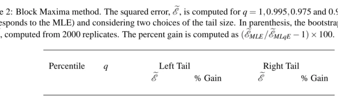
Table 2: Block Maxima method. The squared error,Ee_{, is computed for q=1,0.995,0.975 and 0.95 (where q=1}

corresponds to the MLE) and considering two choices of the tail size. In parenthesis, the bootstrap standard error ofEe, computed from 2000 replicates. The percent gain is computed as(Ee_MLE/Ee_MLqE−1)×100.

Percentile q Left Tail Right Tail

e E _{% Gain} Ee _{% Gain} 1.000 0.3836(0.0332) / 0.2759(0.0248) / 90th 0.995 0.3642(0.0320) 5.3155 0.2716(0.0244) 1.5981 0.975 0.2981(0.0273) 28.6603 0.2565(0.0227) 7.5647 0.950 0.2373(0.0231) 61.6476 0.2429(0.0210) 13.5677 1.000 1.3706(0.1135) / 0.5583(0.0531) / 95th 0.995 1.3213(0.1128) 3.7305 0.5449(0.0523) 2.4618 0.975 1.1594(0.1025) 18.2168 0.4971(0.0478) 12.3238 0.950 1.0239(0.0953) 33.8575 0.4505(0.0432) 23.9352

small. Such settings are typical in finance, where the attention is often on estimating very small probabilities with a small number of extrema. Although we have considered the MLqE for the specific purpose of Extreme Value Theory estimation, this stream of research seems to be very promising, due to the considerable flexibility of the new estimator to many classical estimation settings and its finite-sample variance reduction properties.

The simulation study has pointed out that the MLqE is more accurate than MLE in estimating tail probabilities for GEV and GP distributions for relatively small and moderate sample sizes. The gain from the MLqE appears to be more remarkable when the target tail probability is smaller. When the sample size is too large relative to the choice of the distortion parameter q, the bias component plays an increasingly relevant role and eventually we observe that the MLqE decreases its accuracy. This indicates that the distortion parameter should approach 1 as the sample size increases in order to preserve the efficiency gain. In addition, smaller values of the distortion parameter q enhance the accuracy attainable in small sample situation by reducing the role played by extreme (and more influential) observations. The findings from the simulation study are also confirmed by the empirical analysis on financial data. We show that for more extreme target quantiles, the MLqE achieves a superior performance in terms of generalization error, when the distortion parameter q is chosen to be smaller than 1.

Even if the arbitrariness of the choice of q could be one of the main critics of the new method, we believe that the main strength of the MLqE derives from the flexibility gained from the choice of such a parameter and further work need to be focused on this issue. Currently, two research directions are under investigation on the choice of

q: (i) theoretical derivation of optimal values of q based on asymptotic theory and (ii) data-driven regularization

Table 3: Peaks-Over-Threshold method. Squared error, Ee_{, for q=1, .995, .975 and .95 (when q=1 we are}

computing the MLE) and two choices of the tail size. In parenthesis, the bootstrap standard error ofEe, computed from 2000 replicates. The percent gain is computed as(Ee_MLE/Ee_{MLqE−1)×100.}

Percentile q Left Tail Right Tail

e E % Gain Ee % Gain 1.000 1.4190(0.1307) / 0.522(0.0622) / 90th 0.995 1.3627(0.1277) 4.1327 0.522(0.0618) 0.0094 0.975 1.1630(0.1107) 22.0158 0.5233(0.0623) -0.2430 0.950 0.9671(0.0933) 46.7225 0.5285(0.0631) -1.2296 1.000 7.0898(0.6909) / 1.7555(0.2685) / 95th 0.995 6.7981(0.6763) 4.2903 1.7452(0.2666) 0.5887 0.975 5.7576(0.5813) 23.1364 1.7103(0.2757) 2.6421 0.950 4.7161(0.4806) 50.3295 1.6814(0.2883) 4.4060

Appendix: Delta Method Calculation

Considerα,α_bn,bandα_en,bdefined as in section 4. Moreover, let xB=B−1∑Bb=1(αˆn,b−α)2and yB=B−1∑Bb=1(αen,b−

α)2_{. By the central limit theorem, for large values of B we have that}

√ B xB yB D →N µ= _µ1 µ2 ,Σ= _{σ11 σ12} σ21 σ22 , (17)

whereµ1=MSE(αˆ_n)andµ2=MSE(αen). We are interested in the limiting distribution of g(xB,yB) =xB/yB when B_→∞. By the Delta Method (e.g., see Ferguson (1996)) we have that

√

B g(xB,yB) D

→Ng(µ),g•(µ)TΣg•(µ), as B_→∞ (18) whereg•(·)is the gradient. In this case we have that

• g(µ)T = _∂ ∂ µ1g(µ),∂ µ2∂ g(µ) T = ₁ µ1,−µµ12 2 , (19) and • g(µ)TΣg•(µ) = ₁ µ1,− µ1 µ2 2 _{σ11 σ12} σ21 σ22 1/µ1 −µ1/µ2 2 = σ11 µ2 2 −2σ12µ1 µ3 2 +σ22µ 2 1 µ4 2 .

Therefore, we obtained that √ B _x B yB D →N _µ1 µ2, σ11 µ2 2 −2σ12µ1 µ3 2 +σ22µ 2 1 µ4 2 , as B_→∞. (20)

References

P. Artzner, F. Delbaen, J. M. Eber, and D. Heath. Coherent measures of risk. Mathematical Finance, 9:203–228, 1999.

A. A. Balkema and L. de Haan. Residual life time at great age. The Annals of Probability, 2:792–804, 1974. C. Brooks, J. Clare, J. Dalla Molle, and G. Persand. A comparison of extreme value theory approaches for

determining value at risk. Journal of Empirical Finance, 22:1–22, 2005.

E. Castillo, J. Mar´ıa, and A. S. Hadi. Fitting continuous bivariate distributions to data. The Statistician: Journal

of the Institute of Statisticians, 46:355–369, 1997.

R. Cont. Empirical properties of asset returns: stylized facts and statistical issues. Quantitative Finance, 1,2: 223–236, 2001.

P. Embrechts, C. Kluppelberg, and T. Mikosch. Modelling extremal events for Insurance and Finance. Applications of Mathematics. Springer, 1997.

T. S. Ferguson. A Course in Large Sample Theory. Chapman & Hall Ltd, 1996.

D. Ferrari and Y. Yang. Estimation of tail probability via the maximum Lq-likelihood method. Technical Report

659, School of Statistics, University of Minnesota, 2007. URL http//:www.stat.umn.edu/∼_dferrari/

research/techrep659.pdf.

R. Fisher and L. C. Tippett. Limiting forms of the frequency distribution of largest or smallest member of a sample.

Proceedings of the Cambridge philosophical society, 24:180–190, 1928.

M. Gell-Mann, editor. Nonextensive Entropy, Interdisciplinary Applications. Oxford University Press, New York, 2004.

M. Gilli and E. Kellezi. An application of extreme value theory for measuring financial risk. Computational

Economics, 2-3:207–228, 2006.

G. H. Givens and J. A. Hoeting. Computational Statistics. Wiley, New Jersey, 2005.

B. V. Gnedenko. Sur la distribution limite du terme d’une serie aleatoire. Annals of Mathematics, 44:423–453, 1943.

S. D. Grimshaw. Computing maximum likelihood estimates for the generalized Pareto distribution. Technometrics, 35:185–191, 1993.

T. Hastie, R. Tibshirani, and J. H. Friedman. The Elements of Statistical Learning: Data Mining, Inference, and

J. R. M. Hosking and J. R. Wallis. Parameter and quantile estimation for the generalized Pareto distribution.

Technometrics, 29:339–349, 1987.

P. J. Huber. Robust Statistics. Wiley Series in Probability. John Wiley and Sons, 1981.

A. F. Jenkinson. The frequency distribution of the annual maximum (minimum) values of meteorological events.

Quarterly Journal of the Royal Meteorological Society, 81:158–172, 1955.

J. Knight, S. Satchell, and G. Wang. Quantitative finance. 3:332–344, 2005.

K. Kuester, S. Mittnik, and M. Paolella. Value-at-risk prediction: A comparison of alternative strategies. Journal

of Financial Econometrics, 4,1:53–89, 2006.

N. A. Lazar. Statistics of Extremes: Theory and Applications. Wiley, England, 2004.

A. McNeil and R. Frey. Estimation of tail-related risk measures for heteroskedastic financial time series: an extreme value approach. Journal of Empirical Finance, 7:271–300, 2000.

A. McNeil and A. Stephenson. evir: Extreme Values in R, 2007. URL http://www.maths.lancs.ac.uk/

∼stephena/. R package version 1.5. S original (EVIS) by Alexander McNeil and R port by Alec Stephenson.

A. McNeil, R. Frey, and P. Embrechts. Quantitative Risk Management: Concepts, Techniques and Tools. Princeton Series in Finance, New Jersey, 2005.

R Development Core Team. R: A Language and Environment for Statistical Computing. R Foundation for Statis-tical Computing, Vienna, Austria, 2006. URLhttp://www.R-project.org.

R. Reiss and M. Thomas. Statistical Analysis of Extreme Values with Applications to Insurance, Finance,

Hydrol-ogy and Other Fields. Birkhauser Verlag, Basel, 1997.

M. A. Ribatet. A users guide to the pot package (version 1.0), 2006. URLhttp://cran.r-project.org.

A. van der Vaart. Asymptotic Statistics. Cambridge University Press, New York, 1998.

R. von Mises. La distribution de la plus grande de n valeurs, in Selected Papers, Volume II, volume 44. American Mathematical Society, Providence, RI., 1954.

Figure 1: GP distribution. Monte Carlo Mean Squared Error ratio computed from B=1000 samples of size n, for

α=0.05,0.01,0.005 and q=0.94. The dashed lines represent 95% confidence bands for the case whenα=0.05.

Figure 2: GP distribution. Monte Carlo Mean Squared Error ratio computed from B=1000 samples of size n, for various values of the distortion parameter (q=0.94,0.96,0.98) and true tail probabilityα=0.01.

Figure 3: GEV distribution. Monte Carlo Mean Squared Error ratio computed from B=1000 samples of size n, for two values of the true tail probability (α =0.01,0.05) and distortion parameter q=0.95. The dashed lines represent 95% confidence bands.

Figure 4: GEV distribution. Monte Carlo Mean Squared Error ratio computed from B=1000 samples of size n, for two values of the distortion parameter (q=0.93,0.95) and true tail probabilityα=0.005. The dashed lines represent 95% confidence bands for the case when q=0.95.

RECent Working Papers Series

The most RECent releases are:

No. 1 THE MAXIMUM LQ-LIKELIHOOD METHOD: AN APPLICATION TO EXTREME QUANTILE

ESTIMATION IN FINANCE (2007) D. Ferrari and S. Paterlini

The full list of available working papers, together with their electronic versions, can be found on