A Resource Aware MapReduce based Parallel SVM for
Large Scale Image Classifications
Wenming Guo1, Nasullah Khalid Alham2, Yang Liu3, Maozhen Li4,5 and Man Qi6
1
School of Software Engineering, Beijing University of Post and Telecommunication, 100876, China 2
Nuffield Department of Clinical Laboratory Sciences, University of Oxford, OX3 9DU, UK 3
School of Electrical Engineering and Information, Sichuan University, Chengdu, 610065, China 4
Department of Electronic and Computer Engineering, Brunel University London, Uxbridge, UB8 3PH, UK 5
The Key Laboratory of Embedded Systems and Service Computing, Tongji University, Shanghai, 200092, China 6Department of Computing, Canterbury Christ Church University, Canterbury, Kent, CT1 1QU, UK
Email: [email protected], Tel: +44 1895 266748, Fax: +44 1895 269782
Abstract
Machine learning techniques have facilitated image retrieval by automatically classifying and annotating images with keywords. Among them Support Vector Machines (SVMs) are used extensively due to their generalization properties. However, SVM training is notably a computationally intensive process especially when the training dataset is large. This paper presents RASMO, a resource aware MapReduce based parallel SVM algorithm for large scale image classifications which partitions the training data set into smaller subsets and optimizes SVM training in parallel using a cluster of computers. A genetic algorithm based load balancing scheme is designed to optimize the performance of RASMO in heterogeneous computing environments. RASMO is evaluated in both experimental and simulation environments. The results show that the parallel SVM algorithm reduces the training time significantly compared with the sequential SMO algorithm while maintaining a high level of accuracy in classifications.
Keywords: Parallel SVM, MapReduce, image classification and annotation, load balancing.
1. Introduction
The increasing volume of images being generated by digitized devices has brought up a number of challenges in image retrieval. Content-based image retrieval (CBIR) was proposed to allow users to retrieve relevant images based on their low-level features such as color, texture and shape. However, the accuracy of CBIR is not adequate due to the existence of a Semantic Gap, a gap between the low-level visual features such as textures and colors and the high-low-level concepts that are normally used by the user in the search process [39]. Annotating images with labels is one of the solutions to narrow down the semantics gap [29]. Automatic image annotation is a method of automatically generating one or more labels to describe the content of an image, a process which is commonly considered as a multi-class classification. Typically, images are annotated with labels based on the extracted low level features. Machine learning techniques have facilitated image annotation by learning the correlations between image features and annotated labels.
Support Vector Machine (SVM) techniques have been used extensively in automatic image classifications and annotations [30-36].The qualities of SVM based classifications have been proven remarkable [21, 26, 40-42]. In its basic form SVM creates a hyperplane as the decision plane, which separates the positive and negative classes with the largest margin [21]. SVMs have shown a high level of accuracy in classifications due to their generalized properties. SVMs can correctly classify data which are not involved in the training process. This can be evidenced from our previous work in evaluating the performance of representative classifiers in image annotation [1]. The evaluation results showed that SVM performs better than other classifiers in term of accuracy. However, the training time of the SVM classifier is notably longer than that of other classifiers.
Numerous real world data mining applications involve millions or billions of data instances where processing the entire dataset is computationally intensive. It has been widely recognized that training SVMs is computationally intensive when the size of a training dataset is large. A SVM kernel usually involves an algorithmic complexity of O (m2n), where n is the dimension of the input and m represents the number of training instances. The computation time in SVM training is quadratic in terms of the number of training instances.
To speed up SVM training, parallel computing paradigms have been investigated to partition a large training dataset into small data chunks and process each chunk in parallel utilizing the resources of a cluster of computers [8, 19, 43, 44, 57, 58]. The approaches include those that are based on the Message Passing Interface (MPI) [3, 19, 38, 49, 50, 53]. However, MPI is primarily targeted at homogeneous computing environments and has limited support for fault tolerance. Furthermore, inter-node communication in MPI environments can create large overheads when shipping data across nodes. Although some progress has been made by these approaches, existing parallel SVM algorithms usually partition large datasets into smaller parts with the same size which can be used efficiently only in homogeneous computing environments in which the computers have similar computing capabilities. Currently heterogeneous computing environments are increasingly being used as platforms for resource intensive parallel applications. One major challenge in using a heterogeneous environment is to balance the computation loads across a cluster of participating computer nodes.
This paper presents RASMO, a resource aware parallel SVM algorithm for large scale image classifications [56]. RASMO builds on the Sequential Minimal Optimization (SMO) algorithm [11] for high efficiency in training and employs MapReduce [9] for parallel computation across a cluster of computers. MapReduce has become a major enabling technology in support of data intensive applications. RASMO is implemented using the Hadoop implementation [20, 23] of MapReduce. The MapReduce framework facilitates a number of important functions such as partitioning the input data, scheduling MapReduce jobs across a cluster of participating nodes, handling node failures, and managing the required network communications. A notable feature of the Hadoop implementation of MapReduce framework is the ability to support heterogeneous environments but without an effective load balancing scheme for utilizing resources with varied computing capabilities. For this purpose a genetic algorithm based load balancing scheme is designed to optimize the performance of RASMO on heterogeneous computing environments.
The RASMO algorithm is designed based on a multi-layered cascade architecture which removes non-support vectors early in the training process and guarantees a convergence to the global optimum [6, 45]. The cascade architecture has received significant attention from the research community due to its high accuracy in data training. RASMO partitions the training data set into smaller subsets and allocates each of the partitioned subsets (data chunks) to a single map task in MapReduce. Each map
function (called mapper) trains a subset of the data in parallel in the first layer. The generated support vectors are combined and forwarded as a training input to the next layer. The process continues until only one set of support vectors is left. The support vectors of the final SVM are used to evaluate the initial data chunks to determine whether further optimizations are required. If a global convergence is not reached at this stage, the whole process will be repeated until the global optimum is reached. The genetic algorithm based load balancing scheme is applied in the first of layer computation in RASMO as this layer is the most intensive part in computation in optimizing the whole training dataset. The resulting support vectors from the first layer computation are used to create the input data for next layers which is usually much smaller in size in comparison with the original training data [46]. The size of each data chunk at the first layer is computed by the load balancing scheme based on the resources available in a cluster of computers such as the computing powers of processors, the storage capacities of hard drives and the network speeds of the participating nodes.
The performance of RASMO is first evaluated in a small scale experimental MapReduce environment. Subsequently, a MapReduce simulator is employed to evaluate the effectiveness of the resource aware RASMO algorithm in large scale heterogeneous MapReduce environments. Both experimental and simulation results show that RASMO reduces the training time significantly compared to a standalone SMO algorithm while maintaining a high level of accuracy in classification. In addition, data chunks
with varied sizes are crucial in speeding up SVM computation in the training process. It is worth pointing out that using different sizes for data chunks has no impact on accuracy in SVM classification due to the structure of the RASMO algorithm in which the training work in the first few layers is merely a filtering process of removing non-support vectors and the resulting support vectors of the last layer are evaluated for a global convergence by feeding the output of the last layer into the first layer.
The rest of this paper is organized as follows. Section 2 reviews related work on SVM parallelization. Section 3 presents the design of the MapReduce based RASMO algorithm. Section 4 details the design of a genetic algorithm for load balancing in heterogeneous Hadoop computing environments. Section 5 evaluates the performance of RASMO in a small scale experimental Hadoop computer cluster. Section 6 further evaluates the performance of RASMO in large scale simulated Hadoop environments. Section 7 concludes the paper and points out some future work.
2. Related Work
SVM training is a computationally intensive process especially when the size of the training dataset is large. Numerous avenues have been explored with an effort to increase efficiency and scalability, to reduce complexity as well as to ensure that the required level of classification accuracy can be maintained.
SVM decomposition is a widespread technique for performance improvement [10, 47, 48]. Decomposition approaches work on the basis of identifying a small number of optimization variables and tackling a set of problems with a fixed size. One approach is to split the training data set into a number of smaller data chunks and employs a number of SVMs to process the individual data chunks. Various forms of summarizations and aggregations are then performed to identify the final set of global support vectors. Hazan et al. [8] introduced a parallel decomposition algorithm for training SVM where each computing node is responsible for a pre-determined subset of the training data. The results of the subset solutions are combined and sent back to the computing nodes iteratively. The algorithm is based on the principles of convex conjugate duality. The key feature of the algorithm is that each processing node uses independent memory and CPU resources with limited communication overhead. Zanghirati et al. [19] presented a parallel SVM algorithm using MPI which splits the problem into smaller quadratic programming problems. The output results of the sub-problems are combined. The performance of the parallel implementation is heavily depended on the caching strategy that is used to avoid re-computation of the previously used elements in kernel evaluation which is considered as computationally intensive. Similarly, MPI based approaches have been proposed for speeding up SVM in training [3, 38, 49, 50, 53]. Whilst good performance improvements can be achieved by MPI based parallelization, these approaches tend to suffer from poor scalability, high overhead in inter-node communication, and limited support for heterogeneous computing environments.
Collobert et al. [5] proposed a parallel SVM algorithm which trains multiple SVMs with a number of subsets of the data, and then combines the classifiers into a final single classifier. The training data is reallocated to the classifiers based on the classification accuracy and the process is iterated until a convergence is reached. However the frequent reallocation of training data during the optimization process may cause a reduction in the training speed. Huang et al. [7] proposed a modular network architecture which consists of several SVMs of which each is trained using a portion of the whole training dataset. It is worth noting that speeding up the training process can significantly reduce classification accuracy due to the increase in the number of partitions. Lu et al. [12] proposed a parallel SVM algorithm based on the idea of partitioning training data and exchanging support vectors over a strongly connected network. The algorithm converges to a global optimal classifier in finite steps. The performance of this solution is depended on the size and topology of network. The larger a network is, the higher communication overhead it will incur. Kun et al. [22] implemented a parallel SMO using Cilk [51] and Java threads. The idea is to partition the training data into smaller parts, train these parts in parallel, and combines the resulting support vectors. However Cilk's main disadvantage is that it requires a shared-memory computer [17].
An interesting alternative is considered and discussed in [3].The work on updating optimality condition vectors is performed in a parallel way leading to a speedup in SVM training. However this approach can incur considerable network communication overhead due to the large number of iterations involved. Another approach utilizes Graphics Processing Units (GPU) for SVM speedup [13]. MapReduce was adopted in this work exploiting the multi-threading capabilities of graphics processors. The results show a considerable decrease in processing time. A key challenge with such an approach lies in the specialized environments and configuration requirements. The dependency of specific development tools and techniques as well as platforms introduces additional, non-trivial complexities.
SVM algorithms rely on the number of support vectors for classification. Removing non-support vectors in an early stage in the training process has proven to be useful in reducing the training time. Dong et al. [14] proposed a parallel algorithm in which multiple SVMs are solved with partitioned data sets. The support vectors generated by one SVM are collected to train another SVM. The main advantage of this parallel optimization step is to remove non-support vectors which can help reduce the training time. Graf et al. [6] proposed a similar parallel SVM algorithm using a homogenous Linux cluster. The training data is partitioned and an SVM is solved for each partition. The support vectors from each pair of classifiers are then combined into a new training dataset for which an SVM is solved. The process carries on until a final single classifier is left. Although the convergence to the global optimum can be guaranteed, partitioning a large dataset into smaller data chunks with the same size can only be effective in a homogeneous computing environment in which computers have similar computing capabilities. Another similar work is presented in [27].
Given the focus that most of the current approaches are primarily focusedon the SVM solver, parallelization using a number of computers may introduce significant communication and synchronization overheads. Frameworks such as MapReduce are believed to provide an effective application scope in this context [18]. Chu et al. [4] capitalized natively on the multi-core capabilities of modern day processors and proposed a parallel linear SVM using the MapReduce framework; batch gradient descent is performed to optimize the objective function. The mappers calculate the partial gradient and the reducer sums up the partial results to update the weights vector. However the batch gradient descent algorithm is extremely slow to converge with some types of training data [21].
It is worth noting that several parallel SVM algorithms are implemented on MapReduce based distributed frameworks. Sun and Fox [54] implemented a parallel SVM based Twister MapReduce framework. In this model, training dataset is divided into subsets. Each subset is trained with a SVM model. The non-support vectors are filtered with SVMs. The support vectors of each SVM are taken as the input of next layer SVMs. The global SVM model is obtained through iteration. Experiments show that the parallel SVM algorithm reduces the training time significantly. However experiments are performed using a small homogenous cluster of 8 nodes. It is clear that without an appropriate scheduling scheme it is hard to achieve an optimal solution in heterogeneous computing environments. In addition it is not clear how the algorithm performs with clusters of hundreds or thousands of nodes. Catak and Balaban [55] implemented a parallel SVM based on the Hadoop MapReduce framework. SVM algorithms are trained in parallel then merge all support vectors in all trained SVMs, and the global SVM model is obtained through iteration Experiments are performed using a small homogenous cluster of 10 nodes. The algorithm relies on Hadoop’s default scheduling scheme. As discussed earlier the current implementation of Hadoop only employs first-in-first-out (FIFO) and fair scheduling with no support for load balancing taking into consideration the varied resources of computers. In comparison with the above algorithms, we designed a genetic algorithm based load balancing scheme to optimize the performance of RASMO in heterogeneous computing environments.
Summarizing, research on parallel SVM algorithms has been carried out from various dimensions, but mainly focuses on specialized SVM formulations, solvers and architectures [6-8, 13]. Although some progress has been made in speeding up SVM computation in training, existing approaches on high performance SVMs are mainly targeted at homogenous computing environments using an MPI based solution. Scalability still remains a challenging issue for parallel SVM algorithms. These challenges
motivated the design of RASMO which targets at a scalable SVM in heterogeneous computing environments empowered with a load balancing scheme.
3. The Design of RASMO
This section starts with a brief description of the SMO algorithm followed by a detailed description of RASMO.
3.1 The SMO Algorithm
The SMO algorithm was developed by Platt [11] and further enhanced by Keerthi et al. [16]. Platt takes the decomposition to the extreme by selecting a set of only two points as the working set which is the minimum due to the following condition:
(1)
whereai is a Lagrange multiplier and y is a class name. This allows the sub-problems to have an analytical solution. Despite the need for a number of iterations to converge, each iteration only uses a few operations. Therefore the algorithm shows an overall speedup of some orders of magnitude [21]. The SMO has been recognized as one of the fastest SVM algorithms available. We define an index set
I which denotes the following training data patterns:
I0
i:yi 1,0ai c
i: yi 1,0 ai c
I1
i: yi 1,ai 0
(Positive Non-Support Vectors)I2
i:yi 1,ai c
(Bound Negative Support Vectors) I3
i:yi 1,ai c
(Bound Positive Support Vectors)
: 1, 0
4 i yi ai
I (Negative Non-Support Vectors)
where c is the correction parameter. We also define bias bupand
b
low with their associated indices as follows: bup min
fi :iI0I1I2
Iup argmini fi blow max
fi :iI0 I3 I4
Ilow argmaxi fi The optimality conditions are tracked through the vector fiin Eq. (2).
i i j l j j j i
a
y
K
X
X
y
f
)
,
(
1 (2)where K is a kernel function and Xi is a training data point. SMO optimizes two
a
ivalues related to upb and blowaccording to Eq. (3) and Eq. (4).
0 1
i n i iy aa2new a2old y2
f1old f2old
(3)a1newa1olds
a2olda2new
(4)where2k(X1,X2)k(X1,X1)k(X2,X2) and s y1y2. After optimizing
a
1 anda
2 ,f
i which denotes the error of the ith training data can be updated according to Eq. (5).( 1 1 ) 1 ( 1, ) ( 2 2 ) 2 ( 2, i) old new i old new old i new i f a a yk X X a a yk X X f (5)
To build a linear SVM, a single weight vector needs to be stored instead of all the training data that corresponds to the non-zero Lagrange multipliers. If the joint optimization is successful, the stored weight vector needs to be updated to reflect the new Lagrange multiplier values. The weight vector is updated according to Eq. (6).
w y a a x y a a x
w new newclipped
new ) ( ) ( 1 1 2 2 , 2 1 (6)
We check the optimality of the solution by calculating the optimality gap between the blow and bup. The algorithm is terminated when blowbup2 as shown in Algorithm 1.
3.2 Cascade SVM
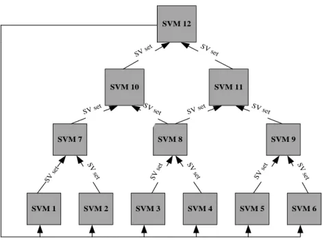
SVM training can be speeded up by splitting the training data set into a number of smaller data chunks and trained separately with multiple SVMs. When the training process is completed, the generated training vectors have support vectors and support vectors. Identifying and removing the non-support vectors in an early stage in the training process is an effective strategy in speeding up SVM [6, 14, 27]. The multilayered cascade architecture follows an approach to derive the global optimum from partial solutions. Figure 1 shows an example of a cascade SVM.
Algorithm 1: Sequential Minimal Optimization
Input: training data xi, labels yi;
Output: sum of weight vector, α array, threshold b and SV; 1: Initialize: αi = 0, fi = -yi;
2: Compute: bhigh, Ihigh, blow, Ilow; 3: Update αIhigh and αIlow; 4: repeat;
5: Update fi;
6: Compute: bhigh, Ihigh, blow, Ilow; 7: Update αIhigh and αIlow; 8: until 2
up low b
b ;
9: Update b;
10: Store the new α1 and α2 values;
Figure 1: A cascade SVM example.
In this architecture a single SVM is trained with a smaller data chunk and non-support vectors are removed. The support vectors generated from one layer are combined as input for the next layer. The process continues until a single set of support vectors is remained. The numbers of the layers depend on the size of training dataset. This architecture insures that SVMs are trained with much smaller training data chunks than the entire training dataset which improves the overall training speed substantially. The cascade architecture is guaranteed to converge to the global optimum as the support vectors of the last layer are fed back into the SVMs in the first layer to determine the level of convergence. In most cases convergence to global optimum is reach with first iteration.
3.3 The RASMO Algorithm
RASMO builds on MapReduce for parallelization of SVM computation in training. We start this section by a brief description of the MapReduce programming model followed by a detailed description of the RASMO algorithm.
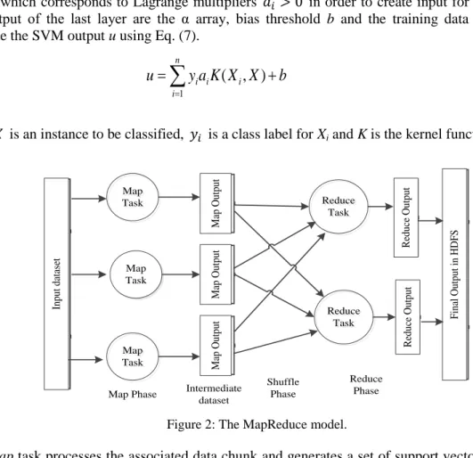
3.3.1 MapReduce Model
MapReduce provides an efficient programming model for processing large data sets in a parallel and distributed manner. The Google File System [15] that underlies MapReduce provides an efficient and reliable data management in a distributed computing environment. The basic function of the MapReduce model is to iterate over the input, compute key/value pairs from each part of input, group all intermediate values by key, then iterate over the resulting groups and finally reduce each group. The model efficiently supports parallelism. Figure 2 shows the workflow of a job in MapReduce. Map
is an initial transformation step in which individual input datasets are processed in parallel. The system shuffles and sorts the map outputs and transfers them to the reducers. Reduce is a summarization step, in which all the associated outputs are processed together.
3.3.2 RASMO Implementation
The RASMO algorithm partitions the entire training data set into smaller data chunks and assigns each data chunk to a single map task. The number of map tasks is equal to number data chunks. Each map
task optimizes a data chunk in parallel in each layer. SVM 1 SVM 12 SVM 11 SVM 10 SVM 9 SVM 8 SVM 7 SVM 5 SVM 4 SVM 3 SVM 2 SVM 6 SV set SV set SV set SV set SV set SV se t layer 1 Layer 2 Layer 3 Layer 4 SV set SV set SV set SV set SV set SV set
The output of each map task is the αarray (Lagrange multipliers) for a local partition and the training data Xi which corresponds to Lagrange multipliers in order to create input for the next layer. The output of the last layer are the α array, bias threshold b and the training data Xi in order to calculate the SVM output u using Eq. (7).
u
y
a
iK
X
iX
b
n i i
)
,
(
1 (7)where is an instance to be classified, is a class label for Xi and K is the kernel function.
In p u t d at as et Map Task Map Task Map Task Map Task Map Task M ap O u tp u t M ap O u tp u t M ap O u tp u t
Map Phase Intermediate dataset Reduce Task Reduce Task Reduce Task Reduce Task Shuffle Phase Reduce Phase R ed u ce O u tp u t R ed u ce O u tp u t F in al O u tp u t in H D F S
Figure 2: The MapReduce model.
Each map task processes the associated data chunk and generates a set of support vectors. Each set of the support vectors is then combined and forwarded to the map task in the next layer as input. The process continues until a single set of support vectors is computed. The set of support vectors of the last layer is then fed back into the first layer together with non-support vectors to determine the level of convergence. The entire process stops when the global optimum is reached indicating that no further optimization is needed in the first layer, and the generated SVM model will then be used in the classification. Figure 3 presents a high level pictorial representation of this approach, in part similar to the approach adopted in [6].
Figure 3: The architecture of RASMO. MR1 Data Chunk 1 MR4 MR3 MR2 MR6 MR5 SV set 1 SV set 2 SV set 3 SV set 4 MR7 Com. Data SV set 5 SV set 6 SVM Com. Data Com. Data Data Chunk 4 Data Chunk 3 Data Chunk 2
Algorithm 2 shows the pseudo code of RASMO with a 3-layer structure. Lines 1-4 show the optimization process of SMO for each data chunk and the combination support vectors of layer 1. Lines 5-8 show the assembling results from layer 1 which are used as input for layer 2. Lines 9-12 show the assembling results from layer 2 which are used as input for layer 1, and the training process in layer 3.
As the entire computation is performed in the map phase, therefore the reduce phase is not required. Having no reduce phase in RASMO further enhances the performance of the algorithm, as the sort, shuffle and reduce phases are known to be computation expensive.
4. The Design of Genetic Algorithm for Load Balancing in Hadoop
A remarkable characteristic of the Hadoop MapReduce framework is its support for heterogeneous computing environments. Therefore computing nodes with different processing capabilities can be utilized to run Hadoop applications in parallel. However, the current implementation of Hadoop only employs first-in-first-out (FIFO) and fair scheduling with no support for load balancing taking into consideration the varied resources of computers. A genetic algorithm based load balancing scheme is designed to optimize the performance of RASMO in heterogeneous computing environments.
4.1 Encoding
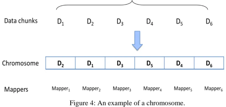
The optimization target is to find an optimal or a near optimal solution for assigning data chunks among the mappers in Hadoop. In genetic algorithms, chromosomes are encoded as a set of strings which are normally binary strings. However, a binary encoding is not feasible as the number of mappers in a Hadoop computer cluster is normally large which will result in long binary strings. As a result, we employ decimal strings to encode chromosomes in the genetic algorithm design. Each data chunk assigned to a mapper is encoded as a gene and
the length of a chromosome
equals to the number of mappers
. The position of a gene represents the sequence number of a mapper which is organized in an ascending order from the left side to the right side in a chromosome. Figure 4 shows a chromosome example with 6 genes.Algorithm 2: RASMO Algorithm Map Tasks
Input: training data xi and label yi;
Output: support vectors svi, threshold bi, data xi and label yi; 1: train SVM on mdata chunks;
2: obtain svm set for mchunks; svm
m 0
;3: combine generated svmsets for each pair of mchunks and corresponding xm;
4: store all xmfor svm to create kinput chunks for the next layer;
5: train SVM on
m
x ;
6: obtain svk set for kchunks; svk k 0;
7: combine svksets for each pair of kchunks and corresponding xk;
8: store all xkfor svk to create input chunk for the next layer; 9: train SVM on xk;
10: obtain svi set for xk; svii0 and bi; 11: evaluate svifor global convergence;
Figure 4: An example of a chromosome.
4.2 Fitness Function
The total time to process data chunks in one processing wave in Hadoop is the maximum time consumed by participating mappers, where
,
According to divisible load theory, to achieve a minimum , it is expected that all the mappers to complete data processing almost at the same time:
Let
be the processing time of the mapper and can be computed following the work presented in [59].
be the average time of the mappers in data processing,
The fitness function measures the distance between Tiand T which can be computed using Eq.(8).
(8)
4.3 Selection
The chromosomes in a population are sorted by their associated fitness values. A better fitness value of a chromosome provides it with a higher probability to survive through the selection step which is based on the roulette wheel method [60]. When a chromosome is added to a new population, it gains a number of slots on the wheel which are associated with the fitness value of that chromosome. Once each chromosome specifies slots on the wheel and the number of chromosomes to be selected for a new generation is set, the wheel can be started spinning. When the wheel stops, a slot will be located. The chromosome associated with the slot will be selected. Usually a chromosome with a larger fitness value occupies more slots on the wheel, which means that the chromosome with a higher statistical probability will be selected to go through the next generation.
D2 D1 D3 D5 D4 D6
Chromosome
Mappers Mapper1 Mapper2 Mapper3 Mapper4 Mapper5 Mapper6
D1 D2 D3 D4 D5 D6
4.4 Crossover
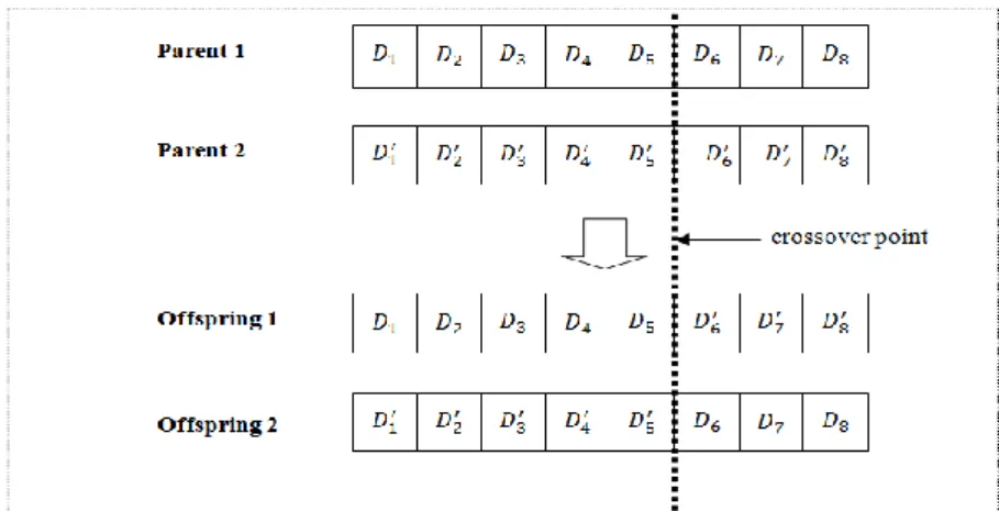
Crossover recomposes the homologous chromosomes via mating to generate new chromosomes which are also called offspring. The generated offspring inherit the basic characteristics of their parents. Some of them may adapt to the fitness function better than their parents do, so they may be chosen as parents in the next generation. Based on crossover, the genetic algorithm can keep evolving until an optimal offspring has been found. In our design, a single-point crossover which refers to setting only one crossover point randomly in the chromosome is employed. The crossover point is randomly generated during the evolution process and the crossover rate is set to 0.6. Figure 5 shows an example of crossover.
Figure 5: An example of crossover.
The process of crossover of the genes in the chromosomes may differentiate the original total volume
of data D = 1 k i i D
. Assume the original total volume of data is 1 k i i D
and the volume of data after crossover is 1 k i i d
, then the difference1 1 k k i i i i D D d
should be considered. In the genetic algorithm, D is divided intok
parts. The size of each part is randomly assigned. And then thesek
parts will be randomly added to or removed from thek
genes in the chromosome. Thus the total size of processed data in one wave can be guaranteed.4.5 Mutation
We conduct a mutation process in the genetic algorithm to avoid a local optimum. In this process, genes are mutated in chromosomes based on a small probability of 0.005. It is similar to the crossover process that the original total volume of data
1 k i i D
may be changed when the value of a gene mutates. Assume the original data volume of the gene is Di and the data volume after mutation isd
i, then the difference
D
D
i
d
i should be taken into account following the way taken in the crossover process.4.6 Termination
The evolution stops if the total number of iterations reaches a predefined number of iterations. The evolution stops if the fittest chromosome of each generation has not changed much, i.e.,
the difference is less than 10-4 over a predefined number.
The evolution stops if all chromosomes have the same fitness values, i.e., when the algorithm has converged.
5. Experimental Results
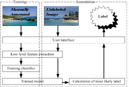
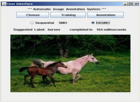
We have incorporated RASMO into our image annotation system which is developed using the Java programming language and the WEKA package [24]. The image annotation system classifies visual features into pre-defined classes. Figure 6 shows the architecture of the system and Figure 7 shows a snapshot of the system. Images are first segmented into blocks. Then, the low-level features are extracted from the segmented image blocks. Each segmented block is represented by feature vectors. We assign the low-level feature vectors to pre-defined categories. The system learns the correspondence between low level visual features and image labels. The annotation system combines low-level MPEG-7 descriptors such as scalable color and edge histogram [25]. In the training stage, the SVM classifier is fed a set of training images in the form of attribute vectors with the associated labels. After a SVM model is trained, it is able to classify a new image into one of the learned class labels in the training set.
Figure 6: Image annotation system architecture.
5.1 Image Corpora
The images are collected from the Corel database [37]. Images are classified into 10 classes, and each class of the images has one label associated with it. The 10 pre-defined labels are people, beach,
mountain, bus, food, dinosaur, elephant, horses, flower and historic item. Typical images with 384x256 pixels are used in the training process. Low level features of the images are extracted using the LIRE (Lucene Image REtrieval) library [28]. After extracting low level features a typical image is represented in the following form:
0,256,12,1,-56,3,10,1,18,...2,0,0,0,0,0,0,0,0,beach
Each image is represented by 483 attributes, and the last attribute indicates the class name which indicates the category to which the image belongs to.
Figure 7: A snapshot of the image annotation system.
5.2 Performance Evaluation
RASMO is implemented using WEKA’s base machine learning libraries written in the Java programming language and tested in a Hadoop cluster. To evaluate RASMO, we extended the SMO algorithm provided in the Weka package, configured it and packaged it as a basic MapReduce job. The Hadoop cluster for this set of experiments consists of a total of 12 physical cores across 3 computer nodes as shown in Table 1.
Table 1: Configurations for an experimental Hadoop cluster. Hardware environment
CPU Number of Cores RAM
Node 1 Intel Quad Core 4 4GB
Node 2 Intel Quad Core 4 4GB
Node 3 Intel Quad Core 4 4GB
Software environment SVM SVM kernels WEKA 3.6.0 (SMO) Polynomial OS Fedora10 Hadoop Hadoop 0.20 Java JDK 1.6
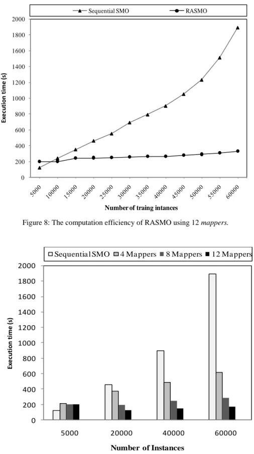
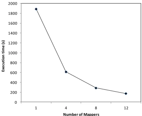
We evaluated the performance of RASMO from the aspects of execution time and accuracy. Figure 8 shows the computation efficiency of the RASMO in SVM training using 12 mappers. The experimental results demonstrate that the sequential SMO is faster than RASMO when the number of training instances is small (e.g. between 5000 and 8000) due to the computation overhead incurred in Hadoop startup. However, RASMO starts to outperform the sequential SMO with an increasing number of instances in terms of training time required. Figure 9 shows that RASMO is highly scalable with a reduction in execution time when the number of participating MapReduce mappers varies from 4 to 12.
Figure 8: The computation efficiency of RASMO using 12 mappers.
Figure 9: The computation efficiency of RASMO in 4 scenarios.
Figure 10 shows that RASMO is scalable with a reduced execution time when the number of participating MapReduce mappers varies from 1 to 12 using 60000 training instances.
0 200 400 600 800 1000 1200 1400 1600 1800 2000 O ve rh ead (s )
Number of traing intances
Sequential SMO RASMO
Ex e cu ti o n ti m e (s ) 0 200 400 600 800 1000 1200 1400 1600 1800 2000 5000 20000 40000 60000 O v er h ea d ( s) Number of Instances
Sequentia l SMO 4 Ma ppers 8 Ma ppers 12 Ma ppers
Ex e cu ti o n ti m e (s )
Figure 10: The computation scalability of RASMO in the experimental environment.
Furthermore we compared the accuracy of RASMO with that of the sequential SMO in classification using 5000 instances. In total 50 unlabeled images were tested (10 images at a time), the average accuracy level was considered. Table 2 shows the comparison results in classification accuracy. It is clear that the parallelization of RASMO has no significant effect on the accuracy level even after the first iteration which is close to the global optimum. The results show that RASMO achieves 94% of correct classifications which is almost the same as the sequential SMO. We have further conducted a 10-fold cross-validation on the two classifiers. The root mean squared errors for the sequential and the parallel classifiers are 0.223 and 0.225 respectively.
Table 2: Classification accuracy.
Sequential SMO RASMO 12 Mappers
Correctly Classified 94.4 % 94.2 %
Incorrectly Classified 5.6% 5.8%
Root Mean Squared Error 0.223 0.225
Total Number of Instances 5000 5000
6. Simulation Results
To further evaluate the effectiveness of RASMO in large scale MapReduce environments, we have implemented HSim [2], a Hadoop MapReduce simulator using the Java programming language. In this section, we assess the performance of the RASMO in simulation environments. Using HSim, we simulated a number of Hadoop environments and evaluated the performance of RASMO in terms of scalability, load balancing effectiveness and overhead of the load balancing scheme.
6.1 Scalability
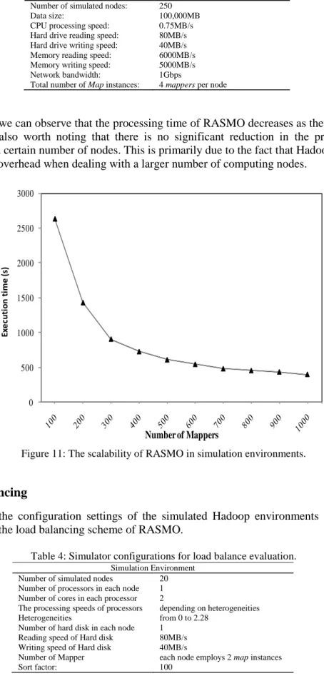
To further evaluate the scalability of the RASMO algorithm, we employed HSim and simulated a number of Hadoop environments using a varying number of nodes up to 250. Each Hadoop node was simulated with 4 mappers, and 4 input data sets were used in the simulation tests. Table 3 shows the configurations of the simulated Hadoop environments.
0 200 400 600 800 1000 1200 1400 1600 1800 2000 1 4 8 12 O ve rhe ad (s ) Number of Mappers Ex e cu ti o n ti m e (s )
Table 3: Simulator configurations for scalability evaluation. Simulation Environment
Number of simulated nodes: 250
Data size: 100,000MB
CPU processing speed: 0.75MB/s Hard drive reading speed: 80MB/s Hard drive writing speed: 40MB/s Memory reading speed: 6000MB/s Memory writing speed: 5000MB/s
Network bandwidth: 1Gbps
Total number of Map instances: 4 mappers per node
From Figure 11 we can observe that the processing time of RASMO decreases as the number of nodes increases. It is also worth noting that there is no significant reduction in the processing time of RASMO beyond certain number of nodes. This is primarily due to the fact that Hadoop incurs a higher communication overhead when dealing with a larger number of computing nodes.
Figure 11: The scalability of RASMO in simulation environments.
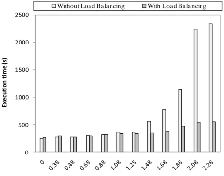
6.2 Load Balancing
Table 4 shows the configuration settings of the simulated Hadoop environments in evaluating the effectiveness of the load balancing scheme of RASMO.
Table 4: Simulator configurations for load balance evaluation. Simulation Environment
Number of simulated nodes 20 Number of processors in each node 1 Number of cores in each processor 2
The processing speeds of processors depending on heterogeneities
Heterogeneities from 0 to 2.28
Number of hard disk in each node 1 Reading speed of Hard disk 80MB/s Writing speed of Hard disk 40MB/s
Number of Mapper each node employs 2 map instances
Sort factor: 100 0 500 1000 1500 2000 2500 3000 O ve r h e ad ( s ) Number of Mappers Ex e cu ti o n ti m e ( s)
To evaluate the load balancing algorithm we simulated a cluster with 20 computing nodes. Each node has a processor with two cores. The number of mappers is equals to the number of cores. Therefore we run two mappers on a single processor with two cores.
The speeds of the processors are generated based on the heterogeneities of the Hadoop cluster. In the simulation environments the total processing power of the cluster was where n
represents the number of the processors employed in the cluster and represents the processing speed of processor. For a Hadoop cluster with a total computing capacity denoted by , the heterogeneity level can be defined using Eq.(9).
(9)
where is the average speed of computers in a Hadoop cluster.
In the simulation, the value of heterogeneity varied from 0 to 2.28. The reading and writing speeds of hard disk were measured from the experimental results. In the RASMO algorithm, mappers are the actual processing units. Therefore balancing the workloads of the mappers in the first layer in the cascade SVM model is the core part of the load balancing algorithm. We employed 10GB data in the tests.
Figure 12 shows the performance of RASMO with load balancing. We can observe that when the level of heterogeneity is less than 1.08 indicating not too heterogeneous environments, the load balancing scheme does not make any difference to the RASMO algorithm in performance. However the load balancing scheme reduces the overhead of RASMO significantly when the level of heterogeneity increases showing that the resource aware RASMO can optimize resource utilization in highly heterogeneous computing environments.
Figure 12: The impact of load balancing with various levels of heterogeneity.
We kept the degree of heterogeneity the same in the simulated cluster but varied the size of data from 1GB to 10GB. This set of tests was used to evaluate how the load balancing scheme performs with different sizes of data sets. Figure13 shows that the load balancing scheme always reduces the overhead of RASMO in SVM training using varied volumes of data.
0 500 1000 1500 2000 2500 O v er h ea d ( s) Heterogeneity
Without Loa d Ba la ncing With Loa d Ba la ncing
Ex e cu ti o n ti m e (s )
Figure 13: The performance of RASMO with a varied volume of data.
6.3 Convergence of the Genetic Algorithm
The load balancing scheme builds on the genetic algorithm presented in Section 4 whose convergence speed affects the computation efficiency of RASMO in training. To analyze the convergence of the genetic algorithm, we varied the number of generations from 1 to 1000 and measured the execution time of RASMO in processing a dataset of 10GB in a simulated Hadoop environment using the configuration settings shown in Table 4. Figure 14 shows that RASMO reaches a stable performance in computation when the genetic algorithm evolves through 300 generations.
Figure 14: Convergence of the genetic algorithm.
0 50 100 150 200 250 300 1 2 3 4 5 6 7 8 9 10 O v e r h e a d (s ) Data size (GB)
Without Load Balancing With Load Balancing
Ex ec uti on ti m e (s ) 0 50 100 150 200 250 300 350 Pe rf o rm a n ce O v er h ea d s o f R A S M O ( s) Number of Generations Ex ec u ti o n t im e o f R A SM O ( s)
7. Conclusion
In this paper we have presented and evaluated RASMO, a resource aware parallel SVM algorithm that capitalizes on the scalability, parallelism and resiliency of MapReduce for large scale image annotations. By partitioning the training dataset into smaller subsets and optimizing the partitioned subsets across a cluster of computing nodes in multiple stages, the RASMO algorithm reduces the training time significantly compared to a standalone SMO algorithm while maintaining high level of accuracy in classification. We introduced a genetic algorithm based load balancing scheme to optimize the performance of RASMO in heterogeneous environment. The load balancing scheme reduces the overhead of RASMO significantly with an increasing levels of heterogeneity showing that the resource aware RASMO can optimize resource utilization in highly heterogeneous computing environments. Both the experimental and simulation results have shown the effectiveness of RASMO in training. To evaluate the scalability of the RASMO algorithm, we employed HSim and simulated a number of Hadoop environments using a varying number of nodes up to 250. We have observed that the processing time of RASMO decreases as the number of nodes increases. We have analyzed the convergence speed of the genetic algorithm in a simulated Hadoop environment. The simulation results have shown that RASMO has a quick convergence process in reaching a stable performance.
We are planning to implement a distributed multiclass SVM algorithm based on one against one technique [52] for high efficiency. For a multiclass problem, it trains all possible binary SVM classifiers which are computationally expensive. The computation task has to be distributed among a cluster of computers. In addition we are planning to consider load balancing scheme in a dynamic heterogeneous environment where the resources and computational capabilities are changed dynamical during Hadoop job execution. We also are planning to evaluate the RASMO on virtualized utility computing environments, such as Amazon’s Elastic Compute Cloud (EC2) to further study the behaviour of the algorithm in cloud environment. Finally we are considering using a much larger number of classes of images to evaluate the performance of the algorithm in terms of classification accuracy and training overhead.
Acknowledgement
This research is partially supported by the National Basic Research Program (973) of China under grant 2014CB340404.
References
[1] Alham N K, Li M, Hammoud S, Qi H (2009) Evaluating machine learning techniques for automatic image annotations, in: Proceedings of the 6th International Conference on Fuzzy Systems and Knowledge Discovery (FSKD), pp 245-249.
[2] Liu Y, Li M, Alham N K, Hammoud S (2013) HSim: A MapReduce simulator in enabling cloud computing, Future Generation Computer Systems, 29(1):300-308.
[3] Cao L, Keerthi S, Chong-Jin O, Zhang J, Periyathamby U, Ju Fu X, Lee H (2006) Parallel sequential minimal optimization for the training of support vector machines, IEEE Transactions on Neural Networks, 17 (4):1039-1049.
[4] Chu C, Kim S, Lin Y, Yu Y, Bradski G, Ng A, Olukotun K (2006) Map-Reduce for machine learning on multicore, in: B. Schölkopf, J.C. Platt, T. Hoffman (Eds.), NIPS, MIT Press, pp 281-288.
[5] Collobert R, Bengio S, Bengio Y (2002) A parallel mixture of SVMs for very large scale problems, Neural Computation, 14(5):1105-1114.
[6] Graf H, Cosatto E, Bottou L, Durdanovic I, Vapnik V (2004) Parallel support vector machines: the cascade SVM, Proceedings of Advances in Neural Information Processing Systems (NIPS).
[7] Huang G, Mao K, Siew C, Huang D (2005) Fast modular network implementation for support vector machines, IEEE Transactions on Neural Networks, 16(6):1651-1663.
[8] Hazan T, Man A, Shashua A (2008) A parallel decomposition solver for SVM: distributed dual ascend using fenchel duality, Proceedings of IEEE Conference on Computer Vision and Pattern Recognition, pp 1-8.
[9] Dean J, Ghemawat S (2008) Mapreduce: Simplified data processing on large clusters, Communications of the ACM, 51(1):107-113.
[10] Osuna E, Freund R, Girosit F(1997) Training support vector machines: an application to face detection, Proceedings of Computer Vision and Pattern Recognition (CVPR), pp 130-136.
[11] Platt J (1998) Sequential minimal optimization: A fast algorithm for training support vector machines, Technical Report, MSR-TR-98-14, Microsoft Research.
[12] Lu Y, Roychowdhury V, Vandenberghe L (2008) Distributed parallel support vector machines in strongly connected networks, IEEE Transactions on Neural Networks, 19(7):1167-1178.
[13] Catanzaro B, Sundaram N, Keutzer K (2008) Fast support vector machine training and classification on graphics processors, Proceedings of the 25th International Conference on Machine learning (ICML), pp 104-111.
[14] Dong J, Krzyżak A, Suen C (2003) A fast parallel optimization for training support vector machine, Proceedings of the 3rd International Conference on Machine learning and Data Mining in Pattern Recognition (MLDM), pp 96-105.
[15] Ghemawat S, Gobioff H, Leung S (2003) The Google file system, Proceedings of Proceedings of the 19th ACM Symposium on Operating Systems Principles (SOSP), pp 29-43.
[16] Keerthi S, Shevade S, Bhattacharyya C, Murthy K (2001) Improvements to Platt's SMO algorithm for SVM classifier design, Neural Computation, 13(3): 637-649.
[17] Kuszmaul B C (2007) Cilk provides the "best overall productivity" for high performance computing: (and won the HPC challenge award to prove it), Proceedings of the 9th ACM Symposium on Parallel Algorithms and Architectures (SPAA), pp 299-300.
[18] Gillick D, Faria A, DeNero J (2012) MapReduce: Distributed Computing for Machine Learning, [Online]http://www.icsi.berkeley.edu/~arlo/publications/gillick_cs262a_proj.pdf. [Last Accessed: 19 May 2015].
[19] Zanghirati G, Zanni L (2003) A parallel solver for large quadratic programs in training support vector machines, Parallel Computing, 29(4):535-551.
[20] Apache Hadoop! [Online]: http://hadoop.apache.org [Last Accessed: 19 May 2015].
[21] Cristianini N, Shawe-Taylor J (2000) An introduction to support vector machines and other kernel-based learning methods, Cambridge University Press.
[22] Kun D, Yih L, Perera A (2003) Parallel SMO for training support vector machines, SMA 5505, Project Final Report.
[23] Venner J (2009) Programming Hadoop, Springer, pp 1-407.
[24] Weka 3, [Online]: http://www.cs.waikato.ac.nz/ml/weka. [Last Accessed: 19 May 2015].
[25] Sikora T (2001) The MPEG-7 visual standard for content description, an overview, IEEE Transactions on Circuits and Systems for Video Technology, 11(6):696-702.
[26] Abe S (2005) Support vector machines for pattern classification (Advances in Pattern Recognition, Springer-Verlag, New York, Inc.
[27] Winters-Hilt S, Armond K (2012) Distributed SVM learning and support vector reduction, [Online]: http://cs.uno.edu/~winters/SVM_SWH_preprint.pdf. [Last Accessed: 19 May 2015]
[28] Lire, An open source Java content based image retrieval library, [Online]: http://www.semanticmetadata.net/lire/ [Last Accessed: 19 May 2015]
[29] Tsai C, Hung C (2008) Automatically annotating images with keywords: a review of image annotation systems, Recent Patents on Computer Science, 1:55-68.
[30] Wong W, Hsu S (2006) Application of SVM and ANN for image retrieval, European Journal of Operational Research, 173(3):938-950.
[31] Gao Y, Fan J (2005) Semantic image classification with hierarchical feature subset selection, in: Proceedings of the ACM Multimedia Workshop on Multimedia Information Retrieval, pp 135-142.
[32] Boutell M, Luo J, Shen X, Brown M (2004) Learning multi-label scene classification, Pattern Recognition, 37(9):1757-1771.
[33] Chen Y, Wang J Z (2004) Image categorization by learning and reasoning with regions, Journal of Machine Learning Research, 5:913-939.
[34] Cusano C, Ciocca G, Schettini R (2004) Image annotation using SVM, Proceedings of SPIE Conference on Internet Imaging, pp 330-338.
[35] Fan J, Gao Y, Luo H, Xu G (2004) Automatic image annotation by using concept-sensitive salient objects for image content representation, Proceedings of the 27th Annual International Conference on Research and Development in Information Retrieval (SIGIR), pp 361-368.
[36] Le Saux B, Amato G (2004) Image recognition for digital libraries, Proceedings of the ACM Multimedia Workshop on Multimedia Information Retrieval (MIR), pp 91-98.
[37] Corel Image Databases, [Online]: http://www.corel.com. [Last Accessed: 19 May 2015].
[38] Bickson D, Yom-Tov E, Dolev D (2008) A Gaussian belief propagation solver for large scale support vector machines, Proceedings of the 5th European Conference on Complex Systems.
early years, IEEE Transactions on Pattern Analysis ana Machine Intelligence,22(12):1349-1380.
[40] Waring C, Liu X (2005) Face detection using spectral histograms and SVMs, IEEE Transactions on Systems, Man, and Cybernetics, Part B: Cybernetics, 35(3):467-476.
[41] Colas F, Brazdil P (2006) Comparison of SVM and some older classification algorithms in text classification tasks, Proceedings of IFIP-AI World Computer Congress, pp 169-178.
[42] Do T, Nguyen V, Poulet F (2008) Speed up SVM algorithm for massive classification tasks, Proceedings of the 4th International Conference on Advanced Data Mining and Applications (ADMA), pp 147-157. [43] Do T, Poulet F (2006) Classifying one billion data with a new distributed SVM algorithm, Proceedings of
the international Conference on Research, Innovation and Vision for the Future (RIVF), pp 59-66.
[44] Chang E Y, Zhu K, Wang H, Bai H, Li J, Qiu Z (2007) PSVM: parallelizing support vector machines on distributed computers, Proceedings of Advances in Neural Information Processing Systems, pp 257–264. [45] Yang J (2006) An improved cascade SVM training algorithm with crossed feedbacks, in: Proceedings of 1st
International Multi-Symposium of Computer and Computational Sciences (IMSCCS), pp 735-738.
[46] Ming-Hsuan Y, Moghaddam B (2000) Support vector machines for visual gender classification, Proceedings of the International Conference on Pattern Recognition (ICOR), pp 5115-5118. [47] Bach F R, Jordan M I (2005) Predictive low-rank decomposition for kernel methods, Proceedings of
the22nd International Conference on Machine Learning (ICML), pp 33-40.
[48] Suykens J K, Vandewalle J (1999) Least squares support vector machine classifiers, Neural Processing Letters, 9(3):293–300 .
[49] Woodsend K, Gondzio J (2009) Hybrid MPI/OpenMP parallel linear support vector machine training, Journal of Machine Learning Research, 10:1937-1953.
[50] Bottou L, Bordes A, Ertekin S (20120 LASVM, [Online]: http://leon.bottou.org/projects/lasvm. [Last Accessed: 19 May 2015].
[51] The Cilk Project, [Online]: http://supertech.csail.mit.edu/cilk/. [Last Accessed: 19 May 2015].
[52] Knerr S, Personnaz L, Dreyfus G (1990) Single-layer learning revisited: a stepwise procedure for building and training a neural network, in: F. Fogelman Soulié and J. Hérault (Eds.) Neurocomputing: Algorithms, Architectures and Applications, volume F68 of NATO ASI Series, pp 41-50, Springer-Verlag.
[53] Cao L J, Keerthi S S, Ong C J, Uvaraj P, Fu X J, Lee H P (2006) Developing parallel sequential minimal optimization for fast training support vector machine, Neurocomputing, 70(1-3): 93-104.
[54] Sun Z, Fox G (2014) Study on Parallel SVM Based on MapReduce, [Online]: http://www.academia.edu/2929779/Study_on_Parallel_SVM_Based_on_MapReduce. [Last Accessed: 19 May 2015].
[55] Çatak F O, Balaban M E (2012) CloudSVM: training an SVM classifier in cloud computing systems. Proceedings of the Pervasive Computing and the Networked World - Joint International Conference (ICPCA/SWS), pp 57-68.
[56] Khalid Alham, N (2011) Parallelizing support vector machines for scalable image annotation, PhD Thesis, Brunel University, UK.
[57] Zhao H X, Magoules F (2011) Parallel support vector machines on multi-core and multiprocessor systems, Proceedings of the 11th International Conference on Artificial Intelligence and Applications (AIA 2011). [58] Zhu-Hong Y, Jian-Zhong Y, Lin Z, Shuai L, Zhen-Kun W (2014) A MapReduce based parallel SVM for
large-scale predicting protein–protein interactions, Neurocomputing, 145:37–43.
[59] Liu Y, Li M, Khan M, Qi M (2014) A MapReduce based distributed LSI for scalable information retrieval, Computing and Informatics, 33(2):259-280.
[60] Goldberg D E (1989) Genetic algorithms in search, optimization, and machine learning, Addison-Wesley, Massachusetts.