Distribution-Dissimilarities in Machine Learning

(1)

Distribution-Dissimilarities

in Machine Learning

Carl-Johann Simon-Gabriel

(2)

(3)

Distribution-Dissimilarities

in Machine Learning

Dissertation

der Mathematisch-Naturwissenschaftlichen Fakultät

der Eberhard Karls Universität Tübingen

zur Erlangung des Grades eines

Doktor der Naturwissenschaften

(Dr. rer. nat.)

vorgelegt von

Carl-Johann P.-M. Simon-Gabriel

aus Neuilly-sur-Seine/Frankreich

Tübingen

2018

(4)

Tag der mündlichen Qualifikation: 17.12.2018

Dekan: Prof. Dr. Wolfgang Rosenstiel

1. Berichterstatter: Prof. Dr. Bernhard Schölkopf 2. Berichterstatter: Prof. Dr. Ulrike von Luxburg

(5)

To my parents, who gave me everything.

To my wife, who became my everything.

(6)

(7)

Abstract

While point-dissimilarities and classifiers are the core of machine learning since its beginnings, distribution-dissimilarities have long seemed a mere theoretical tool for statistical proofs. But both are closely connected: training a binary classifier – more precisely, a score-function – indeed amounts to computing a distribution-dissimilarity. The smaller the classifier’s capacity, the weaker the resulting dissimilarity. Almost all usual dissimilarities are classifier-based. But they happen to be extremely strong: total variation, Hellinger distance, KL-divergence, etc. Weakening them has many advantages: they can get easier to compute and stop saturating on samples. But only up to a certain point, after which they also stop providing enough discrimination. So, what is the right capacity?

We study this question first on maximum mean discrepancies (MMD), a class of weakened total variation dissimilarities. We show that they stay perfectly discriminative if and only if the classifier has enough capacity to approximate a unit ball of continuous functions. Surprisingly, in that case, and only that case, the dissimilarity also stays strong enough to metrize the weak convergence of probability measures. Similar results are provided for what we calltargetedconvergence, as opposed toglobalconvergence. We then provide straight-forward applications in the context of probabilistic programming and the estimation of functions of random variables. We also show that MMDs can be extended from probability measures to generalized measures, called Schwartz-distributions. They en-able us to work with derivatives of probability measures, even when those measures are discrete, like any empirical measure. This leads to new results on kernel Stein discrepancies, an MMD specifically designed for sample-quality tests.

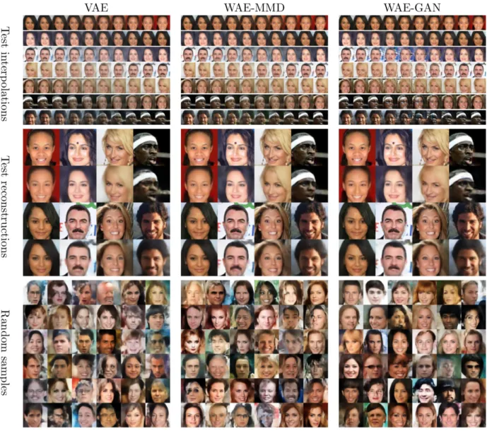
We then turn towards generative models. Contrary to their usual presentation, we introduce several popular models – GANs, VAEs, etc. – as a dissimilarity minimization task. All of them, we will see, minimize approximatef-divergences. So we complement them with another family of distribution-dissimilarities: optimal transport metrics. Our approach leads toWasserstein auto-encodersand unveils new links between VAEs and GANs.

Finally, we focus on two specific deficiencies of the weak distribution-dissimilarities used in genera-tive modeling: mode-collapse and adversarial examples. Mode-collapse is a state where the generator produces only samples of a specific type, ignoring the overall data-diversity. We propose an AdaBoost-like solution calledAdaGAN. It trains several generators sequentially. Each new generator views an automatically reweighted dataset that focuses only on regions not covered by the previous generator. After training, the generators get combined into a single, diversified generative mixture.

As for adversarial examples, they are targeted, but typically imperceptible sample perturbations, that can break even the most accurate classifiers. Because most distribution-dissimilarities used in generative modeling are classifier-based, adversarial vulnerability shows that they are far from a human-like dissimilarity: two almost identical samples can look completely different to them. We explain why. Contrary to human perception, where higher resolution helps, we show, both empir-ically and theoretempir-ically, that the adversarial vulnerability of feed-forward networks increases as the square-root of the input-dimension, almost independently of the architecture. Our findings strongly suggest that, to build robust classifiers and dissimilarities with human-like perception, we need to significantly rethink our network architectures.

(8)

Punktdissimilaritäten und Klassifikatoren sind seit Anfang Kernbestand des maschinellen Lernens. Verteilungsdissimilaritäten dagegen blieben lange nur ein theoretisches Werkzeug für statistische Be-weise. Dabei sind beide eigentlich kaum trennbar: wer einen binären Klassifikator trainiert, genauer gesagt, dessen Score-Funktion, der berechnet eigentlich eine Verteilungsdissimilarität. Je kleiner die Kapazität des Klassifikators, desto schwächer die daraus resultierende Dissimilarität. Nahezu alle üblichen Dissimilaritäten sind klassifikatorbasiert: Gesamtvariation, Hellingerdistanz, KL-Divergenz, etc. Aber sie sind auch außerordentlich stark. Sie zu schwächen, hat viele Vorteile: sie werden oft ein-facher zu berechnen und schwieriger zu sättigen. Doch schwächt man sie zu sehr, so sorgen sie nicht mehr für genügend Diskriminierung. Was, also, ist die richtige Schwächung, die richtige Kapazität des zugrundeliegenden Klassifikators?

Wir untersuchen diese Frage zunächst anhand von MMDs (engl. maximum mean discrepancies), einer Klasse von geschwächten totalen Variations Dissimilaritäten. Wir beweisen, dass MMDs genau dann perfekt diskriminierend sind, wenn der Klassifikator über genügend Kapazität verfügt, um eine Einheitskugel kontinuierlicher Funktionen zu approximieren. Überraschenderweise bleibt auch genau dann die Dissimilarität stark genug, um die schwache Konvergenz über Wahrscheinlichkeits-maße zu dominieren. Ähnliche Ergebnisse liefern wir auch für das neu eingeführte Konzept der gezieltenKonvergenz (statt der üblichen,globalenKonvergenz). Anschließend werden Anwendungen im Rahmen der probabilistischen Programmierung und Schätzung von Funktionen von Zufallsvari-ablen geboten. Nebenbei stellen wir fest, dass MMDs sich leicht von Wahrscheinlichkeitsmessungen auf Schwartz-Verteilungen verallgemeinern lassen. Letztere ermöglichen es, mit Ableitungen von Wahrscheinlichkeitsmaßen zu arbeiten, und zwar auch von diskreten Maßen. Dies führt zu neuen Ergebnissen über Kernel-Stein-Diskrepanzen, also bestimmte MMDs, die speziell zur Anpassungs-gütetests gedacht sind.

Danach wenden wir uns generativen Modellen zu. Im Gegensatz zu ihrer üblichen Präsentation führen wir gängige Modelle wie GANs und VAEs als Dissimilaritätminimierungsmodelle ein. Sie alle minimieren nämlich approximativef-Divergenzen. Wir ergänzen diese Modelle mit einer weiteren Klasse von Dissimilaritätminimierungsmodellen: solche, die optimale Transportmetriken minimieren. Unser Ansatz führt zu Wasserstein Auto-Encodern und enthüllt neue Verbindungen zwischen VAEs und GANs.

Schließlich konzentrieren wir uns auf zwei spezifische Defizite solcher Verteilungsdissimilaritäten, die bei generativen Modellen verwendet werden: Modus-Kollaps (engl. mode-collapse) und gegner-ische Beispiele (engl. adversarial examples). Modus-Kollaps ist ein Zustand, in dem der Generator nur noch Proben eines bestimmten Typs erzeugt und dabei die gesamte Datendiversität ignoriert. Wir schlagen eine AdaBoost-ähnliche Lösung vor: AdaGAN. Dabei werden nacheinander mehrere Generatoren trainiert. Für jeden Generator wird der Datensatz automatisch so neu gewichtet, dass er sich nur auf jene Bereiche konzentriert, die nicht durch die vorherigen Generatoren abgedeckt wur-den. Nach dem Training werden die Generatoren zu einem einzigen, diversifiziertem, generativen Modell zusammengefügt.

(9)

| ix

Bei gegnerischen Beispielen geht es um gezielte, meist aber nicht wahrnehmbare Veränderun-gen der Eingangsdaten, die selbst die besten neuronalen Klassifikatoren verwirren können. Da die meisten Verteilungsdissimilaritäten generativer Modelle auf solchen Klassifikatoren beruhen, be-weisen gegnerische Beispiele, dass solche Dissimilaritäten kaum der menschlichen Wahrnehmung entsprechen. Wir erklären, warum. Beim Menschen hilft es, Bilder in höherer Auflösung zu se-hen. Bei feed-forward Netzwerken dagegen zeigen wir sowohl empirisch als auch theoretisch, dass deren gegnerische Verletzlichkeit mit der Quadratwurzel der Datendimension zunimmt, ziemlich un-abhängig von der Netzwerkarchitektur. Unsere Ergebnisse deuten nachdrücklich darauf hin, dass auf Netzwerk beruhende Klassifikatoren und Dissimilaritäten eine menschenähnliche Wahrnehmung nur bekommen könnten, indem wir deren Netzwerkarchitekturen neu überdenken.

(10)

Writing a thesis is an incredible opportunity. I could dedicate four entire years to what I probably like most: learning and thinking about fascinating new problems. But it would not have been possible and certainly less fun without so many fantastic people around, which I would like to thank here. In particular:

Bernhard Schölkopf, for his constant trust and support, without which this thesis would never have been possible;Ulrike von Luxburg, who was always available when I needed council;Google, and the French and German tax payers, for their generous financial support during my studies and my PhD; Ilya Tolstikhin, with whom I shared not only a room, but also many stimulating discussions and beautiful moments;David Lopez-Paz, who always seemed to believe in me, and convinced me to apply to Facebook AI Research for an amazing internship;Yann Ollivier, who, despite his tight schedule and seniority, always found time to fruitfully help me right down to the slightest details of our common research;Léon Bottou, a man with visions and the patience to share them;Olivier BousquetandSylvain Gelly, for being so reliable, available, and involved in our common projects; Lester Mackey, for his precious and kind guidance on kernel Stein discrepancies; Jonas Peters, always ready to proof-read my papers and their bibliography, and constantly pushing me both in music and teaching; Edgar Klenske, for kindly providing his thesis’ source file as template for this work; and so many other fabulous collegues, collaborators and friends such as Mateo Rojas-Carulla, Tatiana Fomina, Sebastian Gomez-Gonzalez, Martin Arjovsky, Motonobu Kanagawa, Paul Rubinstein, Krikamol Muandet, Diego Fiovaranti, Arthur Gretton, Manuel Gomez-Rodriguez, etc.

Of course, it is one thing to acknowledge the support I got during my thesis, but it would be ungrateful not to mention those that prepared its foundations; in particular my wonderful “prépa” teachers,Frédéric Cuvellier,Thierry Meyer,Frédéric Paviet-SalomonandPatrick Génaux, all extraordinary in their way; and my primary school teachers, Frau Christeaand Madame Garry, who taught me the joys of study and work.

And last but not least, there are no words to thank my family, my parents and my wife. Their love rendered all the rest... Merci.

(11)

6.1 From Adversarial Examples to Large Gradients 94 6.2 Gradient and Adversarial Vulnerability Estimation 97 6.3 Empirical Results 100 6.4 Chapter Conclusion 104 Conclusion 107 Appendix 113 A Background Material 115 A.1 Schwartz-Distributions 115 A.2 Topological Vector Spaces 118 B Details and Chapter Complements 121

B.1 Chapter3 121 B.2 Chapter5 122 B.3 Chapter6 129 C Proofs 135 C.1 Chapter1 135 C.2 Chapter2 141 C.3 Chapter3 151 C.4 Chapter5 155 C.5 Chapter6 162 Bibliography 168 List of Figures 177 List of Tables 177

(13)

Abbreviations & Acronyms

R

spd integrally strictly positive definite AAE adversarial auto-encoder

AVB adversarial variational Bayes

CelebA dataset of celebrity faces with some attributes

CIFAR-10 dataset with 10 classes from the Canadian Institute For Advanced Research CNN convolutional neural network

cpd conditionally positive definite GAN generative adversarial network i.e. id est

iff if and only if

iid independent and identically distributed ImageNet dataset with 1000 classes

IPM integral probability metric JS Jensen-Shannon (divergence) KL Kullback-Leibler (divergence) KME kernel mean embedding

KPP kernel probabilistic programming loc. cv. locally convex

ML machine learning MLP multi-layer perceptron MMD maximum mean discrepancy

MNIST digit dataset from the Mixed National Institute of Standards and Technology OT optimal transport/trasnportation

R.V. random variable resp. respectively

RGB Red-Green-Blue (for colored images) s.t. such that

SGD stochastic gradient descent SNR signal-to-noise ratio spd strictly positive definite

TV total variation (metric/divergence) TVS topological vector space

UGAN unrolled generative neural network VAE variational auto-encoder

WAE Wasserstein auto-encoder

WGAN Wasserstein generative adversarial network wrt with respect to

(14)

Points, Vectors, Sets and Vector Spaces C Complex numbers

E Locally convex, Hausdorff, topological vector space N Non-negative integers

p Element ofNd _{and/or path in a (network-) graph}

R Real numbers

X,Z,Y Arbitrary sets, equipped with a Hausdorff topology and the Borel sigma-algebra. Usu-ally: input, latent and output/label space resp.

x,y,z, ... Scalar or arbitrary points

x,y,z, ... Typically Vectors X,Y,Z, ... Random variables Functions and Function Spaces

1,1S Constant function1, and indicator function of setSresp.

f Real-valued convex function s.t.f(1) =0, used to define anf-divergence

G Generator function (usually defined by a network, for GAN-, VAE-like algorithms) k,kx,kz,kxy Mercer kernels, defined over an arbitrary input space,X,Z, andX×Yresp.

κ Stein kernel derived from kernelk

L Loss function

µk_X,µˆk_X Kernel mean embedding of random variableXw.r.t. kernelk, and its estimator Φk(P) Kernel mean embedding of distributionPw.r.t. kernelk

ϕ Scalar-valued test function

C,C_b Continuous (resp. and bounded) scalar-valued functions Cm_,_Cm

b Scalar-valued, m-times continuously differentiable functions (resp. with all their

partial-derivatives bounded up to orderm) CX _{All functions from}_X_to_C

F Topological vector space of scalar-valued functions.

Fdiv Set of (convex)f-divergence functionsf: (0,∞)→ Rs.t.f(1) =0

G Set of attainable generator functions

H,Hk Reproducing kernel Hilbert space (RKHS) with kernelk

Lm Lebesgue-space ofm-integrable functions Distributions and Distribution Spaces

D Arbitrary (sub)set of Schwartz-distributions

Dm _{Schwartz-distributions of order}_m

Dm

L1 Integrable Schwartz-distributions of orderm: dual ofC

m b

(15)

| xv

Em _{Schwartz-distributions of order}_m_{with compact support: dual of}_Cm

Γ(PX,PY) Couplings (i.e. joint probability distributions) whose marginal laws arePXandPY

Mc Signed measures with compact support

Mδ Signed measures withfinitesupport

Mf Signed finite measures

Mr Signed regular measures

N X;α,σ2

Random variableXfollowing a Gaussian distribution with meanαand varianceσ2

P Probability measures

P,Q Arbitrary probability distribution

p,q,pX Density of distributionsP,Q&PXresp. w.r.t. the Lebesgue measure

dP,dQ Density of distributionsP&Qw.r.t. an arbitrary reference measureµ

PX,PX,Y Probability (resp. joint probability) distribution of random variableX(resp.(X,Y))

P_X_|_Y,Q_X_|_Y Conditional probability distribution ofXgivenY X∼P Random variableXhas distributionP

X_⊥_⊥Y Random variablesXandYare indendent

EP[ϕ(X)] Expectation of random variableϕ(X)whenX∼P

VarX Variance of random variableX

sQ KSE score function with target-densityq

Norms, Distances, Dissimilarities

|x|,|p| Module of scalarx, &Pdi=1piifp= (p1,. . .,pd)∈Nd k·k,_k·kp,_k·kk Arbitrary-,`p-, and RKHS- (with kernelk) norms

|||·||| Dual norm ofk·k

h·,_·i,h·,_·ik Arbitrary and RKHS inner products

kP_kk,hP,Q_ik RKHS norm and inner products of the kernel mean embeddings ofPandQ D(P_kQ) Arbitrary dissimilarity between probability distributionsPandQ

MMDk(P,Q) Maximum mean discrepancy betweenPandQw.r.t. kernelk, i.e.kP−Qkk

KSDk,P(Q) Kernel Stein discrepancy betweenQand targetP, i.e. MMDκ(P,Q).

Pn→bP,Pn→σP,Pn→wP,Pn →k·kk,Pn→αP

Convergence of (Pn)n to P in bounded, weak, weak-*, RKHS and Wasserstein-α

topologies resp. See Table1.2and Prop.3.1.1

Miscalleneous

∂xϕ,∂pϕ partial derivative ofϕw.r.t.x& ∂

|p|_f

∂p1x1∂p2x2···∂pdxd, wherep= (p1,. . .,pd)∈N

d ∂ϕ,∂xϕ gradient & gradient w.r.t. vectorxof functionϕ

domϕ Input domain of functionϕ

dp Path-degree vector of pathpin a network

P(x,o) Set of all pathspfrom nodexto nodeo

D(x,o) set of path-degree vectors for all paths going from nodexto nodeo. Fϕ Fourier transform ofϕ

spanS Linear span of setS

E1,→E2 Continuous inclusion, i.e.E1⊂E2and the canonical embedding is continuous

(16)

(17)

(18)

(19)

introduction | 3

F

our years ago, Goodfellow et al. [37] proposed a new algorithm [37] Goodfellow et al.,Generative

Adver-sarial Nets, 2014

that gained instant popularity: Generative Adversarial Nets (GANs). To generate fake but realistically looking data, they pro-posed to use two networks – a generator and a discriminator – with opposite goals: the discriminator tries to distinguish true from fake data, while the generator produces fake data that tries to fool the discriminator. Both networks permanently evolve while adapting to the strengths and weaknesses of each other until the generator starts producing realistic data.

Remarkably, GANs do not need any predefined measure to quan-tify what it means to “look realistic” – or so it seems. Where previous algorithms used refined, closed-form dissimilarity measures such as the KL-divergence or the total variation between fake and true prob-ability distributionsP andQ, GANs judge the quality ofPby their discriminator’s ability to distinguish it from Q. They optimizePto minimize the average reward of a (logit-) discriminator ϕ trained over a set of functions Fto distinguishPfrom Q. It turns out that the maximal average reward of ϕis a distribution-dissimilarity too: we call it a classifier-based dissimilarity. For a loss function L (the negative reward), it can formally be written as

GANs Minimize a Classifier-Based Dissimilarity D_L_,_F_,_π(P_kQ) := sup

ϕ∈FXE,C

−L(ϕ(X),C), (0.1) where(X,C)denotes a sampleXcoming fromPifC= 1 and from

QifC=0, and whereπis the (prior) probability thatC=1.1 1 The dependence onπbecomes clear when noting thatEX,CL(ϕ(X),C) =

πEXL(ϕ(X),1)+

(1−π)EXL(ϕ(X),0).

Classifier-based dissimilarities are extremely general: by varying

L, F and π, one covers all integral probability metrics (IPMs) and f-divergences. That includes the KL-, reverse KL-, Jensen-Shannon-and squared-Hellinger divergences, the total variation-, Wasserstein-1-, Dudley- and maximum mean discrepancy (MMD) distances, etc. The original GAN algorithm used a logistic loss Landπ = 1_/2. In

that caseD_L_,_F_,πhappens to approximate the Jensen-Shannon

diver-gence more and more accurately with growing capacity of F. But

could we use otherf-divergences or IPMs as proposed by [82]? What [82] Nowozin et al.,f-GAN, 2016

would be the pros and cons? More generally:

What are the properties of such distribution-dissimilarities? What are they good for?

This is the core question which serves as leitmotiv to the present the-sis. Rather than trying to answer it exhaustively, we will focus on the properties of someselecteddistribution-dissimilarities and present se-lectedapplications, GANs being only one of them. Now, we propose to give a brief overview of the major distribution-dissimilarities that we will encounter throughout this thesis and then present the con-tents of the chapters to come.

(20)

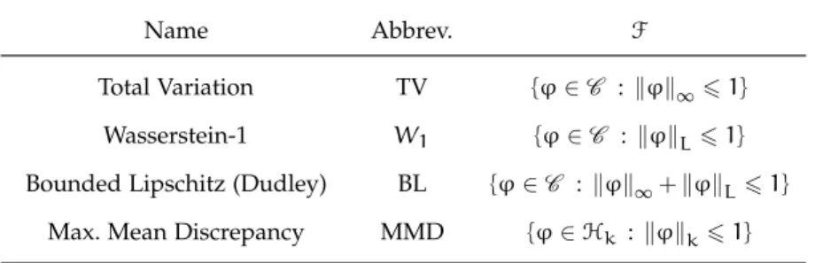
Name Abbrev. F

Total Variation TV {ϕ_∈C : kϕk_∞61}

Wasserstein-1 W1 {ϕ∈C : kϕkL61}

Bounded Lipschitz (Dudley) BL {ϕ_∈C : _kϕ_k_∞+_kϕ_kL61}

Max. Mean Discrepancy MMD {ϕ_∈Hk : kϕkk61}

Table 0.1: IPM examples. k·k_∞, k·k_∞ and k·k_k denote the supremum, the Lipschitz and an RKHS norm (of RKHS Hkwith kernelk) respectively.

0.1

Distribution Dissimilarities

Let Xbe the input space, typically a Polish space (separable, com-plete and metrizable) equipped with its Borel sigma-algebra. We

Definition of Distribution-Dissimilarity call distribution-dissimilarityor simply dissimilarity any real function

D of two probability distributionsP,Q defined onXthat gets mini-mized when P = Q. D(P_kQ) is typically non-negative and equal to 0 when P = Q, but not necessarily. We will encounter three big families of distribution-dissimilarities: Integral Probability Met-rics (IPMs), f-divergences, and Optimal Transport (OT) dissimilari-ties. Let us present them here, and then see how they relate to the classifier-based dissimilarity (0.1).

0.1.1

Textbook Dissimilarities

There are several ways to present IPMs, f-divergences and OT dis-similarities. They can usually be defined using either their primal or their dual formulation. Both are equivalent. Here, we opt for the more unusual dual definitions, so as to make the link between all three dissimilarity families appear more explicitly. Indeed, all of them can be written as

IPMs,f-Divergences and OT Dissimilarities All Verify(0.2). D(P_kQ) = sup

(ϕ,ψ)∈(F,G)

P(ϕ) −Q(ψ), (0.2) where P(ϕ)is a short-hand for EX∼Pϕ(X)and (F,G)denotes a set

of measurable function pairs (ϕ,ψ) such that ϕ and ψ are P- and Q-integrable respectively.

Integral Probability Metrics (IPM) correspond to(F,G) ={(ϕ,ϕ) : ϕ_∈F}, whereFis some fixed (usually balanced) set of functions.

D_F(P_kQ) = sup

ϕ∈F

P(ϕ) −Q(ϕ). (0.3) IPMs satisfy the axioms of a metric (or distance), except that they may take infinite values (D_F(P_kQ) = ∞) and need not be definite,

id est (i.e.) perfectly discriminative.2 Various IPM examples are given 2Definite(orperfectly discriminative) dis-similarity: D_F(PkQ) = 0 ⇒ P = Q.

(21)

distribution dissimilarities | 5

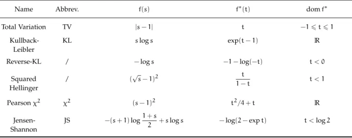
Name Abbrev. f(s) f∗(t) domf∗

Total Variation TV |s−1| t −16t61

Kullback-Leibler

KL slogs exp(t−1) R

Reverse-KL / −logs −1−log(−t) t < 0

Squared Hellinger / (√s−1)2 t 1−t t < 1 Pearsonχ2 χ2 (s−1)2 t2/4+t R Jensen-Shannon JS −(s+1)log1+s

2 +slogs −log(2−expt) t <log2

Table 0.2: Examples of f-divergences, withf, its Fenchel conjugatef∗and the latter’s input domain domf∗. Taken from [82]

f-Divergences correspond to (F,G) = {(ϕ,f∗(ϕ))} where f : (0,∞)_→ R is any fixed convex function satisfying f(1) = 0, f∗ is

its Fenchel conjugate,3 and whereϕ spans the set of all measurable 3 Fenchel conjugate definition:

f∗(t) :=sups∈domfst−f(s)

functions fromXto the input domain domf∗off∗. See [82] & [85].

[82] Nowozin et al.,f-GAN, 2016 [85] Peyré and Cuturi, Computational Optimal Transport, 2018, Rmk 8.1 D_f(P_kQ) = sup

ϕ:X→domf∗

P(ϕ) −Q(f∗(ϕ)) (0.4) f-divergences may not satisfy the triangular inequality, but they are always non-negative and definite. Examples off-divergences include the Kullback-Leibler (KL), reverse-KL, Jensen-Shannon (JS), squared Hellinger and χ2-divergences, and the TV distance. The latter cor-responds to f∗(x) = x for−1 ₆ x ₆ 1. It is the onlyf-divergence that is also an IPM. There are many connections between the differ-entf-divergences, and betweenf-divergences and statistical informa-tion [67].

[67] Liese and Vajda,On Divergences and Informations in Statistics and Information Theory, 2006

Optimal transport (OT) dissimilarities correspond to (F,G) =

{(ϕ,ψ) : _∀x,y _∈ X,ϕ(x) +ψ(y) ₆ c(x,y)}, where c(x,y) is any predefined, non-negative cost function. It is usually interpreted as the cost of transporting a unit mass from pointxto pointy.

D_c(P_kQ) = sup

(ϕ,ψ):∀x,y∈X

ϕ(x)+ψ(y)6c(x,y)

P(ϕ) −Q(ψ)

In general, optimal transportation measures satisfy neither definite-ness, nor the triangular inequality, but they are always non-negative and finite ifcis. Whencis a distance, thenDc(and more generally

D1_c/pp) also satisfies the axioms of a distance, except that it may take

infinite values. It is called the c-Wasserstein-1 (resp. c -Wasserstein-p) distance, or simply the Wasserstein-1 distance when c coincides with the underlying metric ofX. Thec-Wasserstein-1 is an IPM,

(22)

co-inciding with the total variation metric when c is the discrete

dis-tance [121]. [121] Villani,Optimal Transport: Old and New, 2009, Chap. 6

0.1.2

Classifier-Based Dissimilarities

How do the previous three dissimilarity families relate to GANs and classifier-based dissimilarities, as discussed in (0.1)? Let us just il-lustrate here the main ideas of the answer on f-divergences. More details and links are given in Chapter4.

The trick is to see every test function ϕ in the definition (0.4) of f-divergences as a score-function. For brevity, we may refer toϕ as the classifier, but it is more accurate to think of it as the logit function of a binary classifier. It takes an inputx_∈Xand tries to determine if xwas drawn from distributionPor fromQ. The higher the score ϕ(x), the more it attributesxtoP. Now, define the reward for score ϕ(x) as ϕ(x) if x comes from P, and −f∗(ϕ(x)) otherwise. Then P(ϕ) −Q(f∗(ϕ)), i.e. EX∼P[ϕ(X)] −EX∼Q[f∗(ϕ(X))], is the average

reward ofϕwhenxcomes with equal probability fromPorQ. And

f-Divergences are Classifier-Based Dissimilarities D_f(P_kQ) is the maximal average reward that we can get when ϕ

is optimized over all functions fromXto domf∗. f-divergences are hence, by definition, classifier-baseddissimilarities. They satisfy (0.1) for the particular choices π = 1_/2 _{(equal prior probability to come}

fromPorQ),F= [−1,1]X:={ϕ:X_→ domf∗}, and

L(ϕ(x),y) =   

−ϕ(x) ify=1 (i.e. ifxcomes fromP) f∗(ϕ(x)) ify=0 (i.e. ifxcomes fromQ). f-divergences are particularly strong dissimilarity measures, be-cause of their huge set of test functions F. As we will see in a mo-ment, that often makes them too discriminative. So we may want to deliberately reduce the set of test functions F. In a sense, we

al-They can be Weakened by Reducing the Set of Test FunctionsF ready did so with IPMs. They are weak total variation dissimilarities,

that replace the set of all measurable functionsϕ: X_→ [−1,1]by a smaller one. Doing the same, not just with total variation, but with anyf-divergence leads torestrictedf-divergences.

Restricted (or approximate)f-divergences have the same objective thanf-divergences, but are optimized over a smaller set of test func-tionsF:

D_f_,_F(P_kQ) = sup

ϕ∈F

P(ϕ) −Q(f∗(ϕ)).

IPMs and f-divergences are thus particular kinds of restricted f -divergences: IPMs fix f and varyF, whilef-divergences keepF as big as possible and varyf. Restrictedf-divergences are in particular

(23)

distribution dissimilarities | 7

classifier-based dissimilarities that restrict the capacity of their score-function set to F. They are hence weaker thanf-divergence, in the sense that

D_f_,_F(P_kQ)₆D_f(P_kQ) .

The lower bound converges to the upper limit whenFgrows towards (domf∗)X. But in practice, we may actually prefer the lower bound; the weaker dissimilarity. Let us explain why.

0.1.3

Why Weak Distribution Dissimilarities?

Probability theory and statistics traditionally work with strong distribution-dissimilarities; probably because they mainly deal with continuous probability distributions and because stronger assump-tions can considerably simplify a proof. But applied machine learn-ing (ML) is mainly about samples, i.e. empirical measures that have no density. We may for example want to do a two sample test, to evaluate if two samples come from a same distribution; or a sample-quality test, that checks if a sample could come from some prede-fined, usually continuous reference distribution. Such tests can be used in the context of MCMC sampling or of generative modeling, such as in GANs. For all of them, distribution-dissimilarities seem the right tool.

But here is the catch. Two random samples typically yield disjoint measures; andf-divergences typically saturate on such measures: to-tal variation for example simply takes its maximal value2; the KL-divergence is even infinite. In a sense, that is not surprising. In theory, the two measures are perfectly distinguishable. So the aver-age reward D_f(P_kQ) of an optimally classifying score-function ϕ is as high as it can get: the dissimilarity saturates. This saturation masks a lot of relevant comparative information. Two distinct Dirac measuresδxandδy, how ever close they are, always lie at the same,

maximal TV-distance, 2. Of course, being distinct, they are theoreti-cally perfectly distinguishable. But it would nevertheless help if the dissimilarity converged to 0 when y _→ x. That is where weaker dissimilarities come into play.

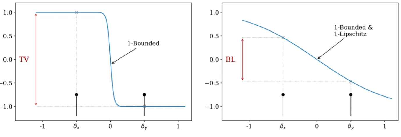
Consider the total variation again, and imagine that, instead of choosing the test-function ϕ among all functions with output in [−1,1], we additionally required that it be 1-Lipschitz. D_F(δxkδy)

gets maximized only if there exists a test-function ϕ _∈ Fsuch that (s.t.) ϕ(x) = 1 and ϕ(y) = −1. As illustrated in Figure 0.1, when

F = [−1,1]X, this is the case as soon as x ₆= y. But if ϕ is to be 1-Lipschitz,|ϕ(x) −ϕ(y)|₆|x−y|. So, not only can’t the condition be met if|x−y|< 2, but the new dissimilarity4D

f

BL(δykδx)converges

4 Technically, this new dissimilarity is not exactly the bounded Lipschitz (Dudley) one defined in Table 0.1, which is why we denote itD

f BL rather thanDBL. But both define equivalent norms, i.e. are “almost the same”.

(24)

-1 x 0 y 1 1.0 0.5 0.0 0.5 1.0 1-Bounded

TV

-1 x 0 y 1 1.0 0.5 0.0 0.5 1.0 1-Bounded & 1-Lipschitz

BL

Figure 0.1: Two test functions ϕ that (almost) achieve supϕ∈Fδx(ϕ) −

δy(ϕ) =D_F(δxkδy)whenF

con-tains resp. all 1-bounded functions (left) and when it contains only 1-bounded 1-Lipschitz functions (right). The first dissimilarity (TV) is bigger than the sec-ond (bounded Lipschitz).

to 0 wheny_→x. We say thatD

f

BLmetrizes a new, weaker topology:5

5 Formally, TV metrizes thestrong con-verges of probability measures, while the bounded Lipschitz dissimilarity metrizes theweakone.

while in total variation, δy_n _→δx if and only if (iff) yn = xfor all

large enoughn, in the new topologyδyn →δxiffyn→x. This new

topology is much more informative, because, in a sense, it respects the underlying topology ofX.

Instead of simply imposing ϕ to be 1-Lipschitz, we could add more restrictions, decreasing F even further. That might ease the training procedure, i.e. the optimization of ϕ inF. But it may also weaken the dissimilarity too much. Imagine for instance that we kept only one single function in F. Then, no need to optimize ϕ anymore. But all distributions are at equal distance: the dissimilar-ity becomes totally uninformative. We hence have to find the right balance between a setFthat is sufficiently small to get a computable dissimilarity measure, but sufficiently large to stay informative.

Of course, what it means to “be informative” depends on our goals. If our only goal is to distinguish true from fake image datasets, we may be content with a dissimilarity that sees no difference be-tween any two different sets of fake images. But if we intend to generate realistic images, we’d better have a dissimilarity that sees differences even in between fake images, and can tell us which one looks more realistic. So the real question, at the core of this thesis, is not so much: how much functions can I take our of F? But rather: given my goals, how should I choose F; how should I choose my distribution-dissimilarity? Our three parts focus on three different aspects of this question.

0.2

Thesis Outline

Our first part focuses on two questions: 1) if I want my dissimilarity to be perfectly discriminative, how should I choose the set of test-functionsF? 2) same question, if I want my dissimilarity to metrize a topology known as weak convergence? We study these questions on a particular family of IPM dissimilarities called maximum mean

(25)

thesis outline | 9

discrepancies (MMDs). Those are weak total variation dissimilari-ties where F is the unit ball of a reproducing kernel Hilbert space (RKHS)Hk. RKHSs are function spaces that are entirely determined

by a (Mercer) kernel (function)k. That gives flexibility: by changing the kernel, we change the RKHS. It also makes RKHSs very rigid, which can be both good and bad. Good, because it can consider-ably easen computations: the MMD of two samples for example can always be expressed in closed form. Bad, because RKHS functions in-herit many properties of the kernel, which can make them relatively small: if k is bounded, continuous, differentiable and/or smooth, then so are all the functions in the respective RKHS. Some RKHSs get so small, that their MMD is far from being perfectly discrimina-tive. Others, however, are still big enough to be dense in the set of bounded continuous functionsCb. Intuitively, that seems enough to preserve perfect discrimination. Chapter1confirms this intuition: it

shows6 that the MMD of a bounded continuous kernel is perfectly 6 Theorem1.2.2 discriminative iff Hk is dense in Cb. More surprising however is

that this condition also happens to be necessary and sufficient to metrize weak-convergence. That is the main theorem of Chapter 1, Theorem1.3.4, and possibly the main theorem of this thesis. Finally, Chapter1 also shows that MMDs can be extended from probability measures to generalized measures calledSchwartz-distributions. That will turn out very useful later on. Chapter2and3then propose two applications: one related to the weak-convergence metrization, and another that makes use of Schwartz-distribution embeddings.

Our second part focuses on distribution-dissimilarities in the con-text of generative models, such as in GANs and variational auto-encoders (VAEs). It implicitly asks: how can I build effective distribution-dissimilarities to learn to generate image data? To do so, Chapter 4 first lists, compares and links the objectives of exist-ing generative algorithms and shows that they all do approximate f-divergence minimization. It then proposes a new, related objective, which implements approximate OT minimization: Wasserstein auto-encoders (WAE). Chapter5then remedies a deficiency of GANs and similar generative algorithms known asmode collapse, where the gen-erator suddenly produces only one kind of datapoints, ignoring the true data diversity. The solution we propose – an algorithm called AdaGAN – can be applied to any generative method that minimizes a restrictedf-divergence.

Our third and final part focuses on an appealing deficiency of all state-of-the-art network-based image-classifiers: their adversarial vulnerability. By adding imperceptible, but targeted perturbations to the input images, the accuracy of almost any such classifier can be drastically turned down. The perturbed and original sample would hence look almost the same to humans, but entirely different to the

(26)

classifier-based dissimilarity. Understanding the origins of adversar-ial vulnerability therefore seems a prerequisite for building dissim-ilarity measures that capture more human-like perception. But we make worrying findings. For humans, higher resolutions can but help. But for feed-forward networks, independently of their archi-tecture, adversarial vulnerability increases as the square-root of the input dimension. This we show both theoretically and empirically. It strongly suggests that, despite their fantastic accuracies, we may want to rethink our network architectures, if they are to imitate, one day, human-like perception.

0.3

Underlying Material, Co-Workers and Contributions

This work relies on the following papers, which have all been co-written with colleagues and friends. I would like to acknowledge and thank them here, and briefly outline the extent of my personal contributions.

Chapter1

C.-J. Simon-Gabriel and B. Schölkopf. Kernel Distribution Em-beddings: Universal Kernels, Characteristic Kernels and Kernel Met-rics on Distributions. In:JMLR(2018). to appear

Contributions:main ideas, and major part of theory and text. Chapter2

C.-J. Simon-Gabriel, A. Scibior, I. O. Tolstikhin, and B. Schölkopf. Consistent Kernel Mean Estimation for Functions of Random Variables. In:NIPS. 2016, pp. 1732–1740

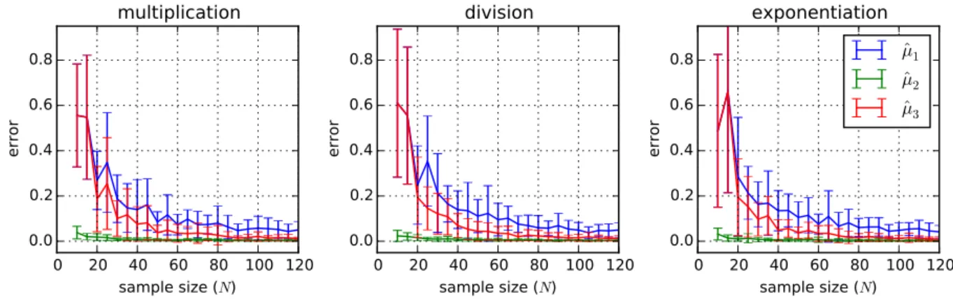
Contributions:a major part of the theory (especially the proofs of the main Theorems 2.2.1&2.2.3) and a substantial part of the text. The code for the little experiment of Figure 2.1was graciously provided by Krikamol Muandet. Compared with the paper, I also shifted the focus from convergence of KME estimators to the convergence of discrete random samples (see Section2.1.2).

Chapter3

C.-J. Simon-Gabriel and L. Mackey. Targeted Convergence Char-acteristics of Maximum Mean Discrepancies and Kernel Stein Dis-crepancies. In:preprint(2018)

Contributions:the original idea of targeted convergence and its application to kernel Stein discrepancies came from L. Mackey, but I worked out most of the theory, proofs and text.

Chapter4

(27)

underlying material, co-workers and contributions | 11

B. Schölkopf. From optimal transport to generative modeling: the VEGAN cookbook. 2017. arXiv: 1705.07642

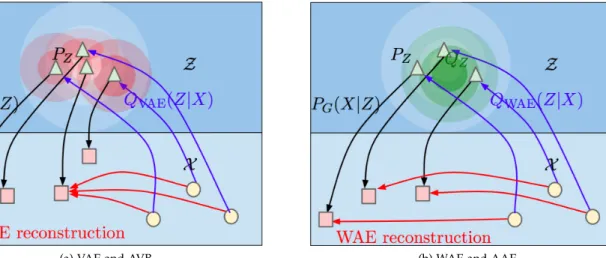
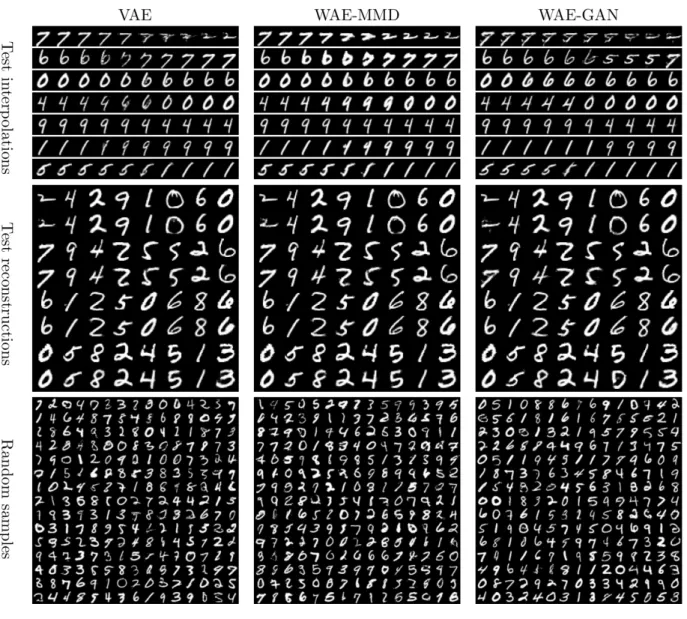
Contributions:I was mainly involved in the initial ideas and ex-periments, and afterwards in the analysis discussions. While I contributed only little to the original text, I significantly modi-fied it for this thesis. The proofs however were mainly O. Bous-quet’s work. I also included experimental results and images

of [116], which is a follow-up paper that further implements [116] Tolstikhin et al.,WAE, 2018

and tests our main algorithm.

Chapter5

I. O. Tolstikhin, S. Gelly, O. Bousquet, C.-J. Simon-Gabriel, and B. Schölkopf. AdaGAN: Boosting Generative Models. In: NIPS. 2017, pp. 5424–5433

Contributions: I contributed to the original idea, the dis-cussions, did a significant part of the experiments, and co-analyzed the results. The proofs however were mainly worked out by I. Tolstikhin and O. Bousquet. The initial idea came from B. Schölkopf during a joint discussion.

Chapter6

C.-J. Simon-Gabriel, Y. Ollivier, B. Schölkopf, L. Bottou, and D. Lopez-Paz. Adversarial Vulnerability of Neural Networks In-creases With Input Dimension. 2018. arXiv: 1802.01421

Contributions:The main ideas resulted from my work and dis-cussions at Facebook AI Research during my internship there. I coded all experiments, and a major part of the theorems and proofs. The idea to generalize Theorem6.2.1and Corol-lary 6.2.3 from fully-connected and standard convolutional nets to general feed-forward nets (Theorem 6.2.2) came from Y. Ollivier. I worked out its proof under his guidance.

This thesis will not study the following co-authored papers:

B. Schölkopf, D. W. Hogg, D. Wang, D. Foreman-Mackey, D. Janzing, C.-J. Simon-Gabriel, and J. Peters.Removing Systematic Errors for Exoplanet Search via Latent Causes. In: ICML. 2015. arXiv:1505.03036

B. Schölkopf, D. W. Hogg, D. Wang, D. Foreman-Mackey, D. Janzing, C.-J. Simon-Gabriel, and J. Peters. Modeling Confound-ing by Half-SiblConfound-ing Regression. In:PNAS113.27 (2016), pp. 7391– 7398

H. Huang, G. M. Peloso, D. Howrigan, B. Rakitsch, C. J. Simon-Gabriel, J. I. Goldstein, M. J. Daly, K. Borgwardt, and B. M.

(28)

Neale. Bootstrat: Population Informed Bootstrapping for Rare Vari-ant Tests. In: (2016). bioRxiv:10.1101/068999

The German abstract (Zusammenfassung) was originally translated

from English with the DeepL Translator [23], and significantly modi- [23] DeepL,DeepL Translator, 2018

(29)

Part I

(30)

(31)

maximum mean discrepancies: introduction | 15

T

his first partfocuses on a very particular class of dissimilarity

measures: maximum mean discrepancies (MMDs). MMDs are

MMDs: A Case Study for Dissimilarity Weakening IPMs, where the test functions ϕ _∈ F are the unit ball of a

repro-ducing kernel Hilbert space (RKHS) Hk with kernel k. We assume

that the reader is familiar with the basics of RKHS theory. For an

introduction, see [94] or [79]. MMDs have many attractive features [94] Schölkopf and Smola,Learning with Kernels, 2001

[79] Muandet et al.,Kernel Mean Embed-ding of Distributions, 2017

– such as being computable in closed form for any two samples – which gave them quick popularity after their introduction in the ML community in the early 2000s. But compared to more classical spaces such as the continuous bounded and/or Lipschitz functions, RKHS are relatively small, as they inherit many properties of their kernel: ifkis continuously differentiable in each variable, so are all the func-tions ofHk; ifx7→ k(x,x)is Lp-integrable, so are the functions ofHk.

This makes the resulting MMD weaker than more classical IPMs such as the total variation, Wasserstein-1 or Dudley distances. Chapter 1 studies how weak (or strong) MMDs actually are.

A first weakness is that MMDs may not be perfectly discrimina-tive – meaning thatD(P_kQ) =0 may not implyP =Q – in which case the MMD is a semi-metric, but not a metric. Chapter 1 hence first focuses on identifying necessary and sufficient conditions for MMDs to be metrics. A second weakness is that the convergence

MMDs, Perfect Discrimination & Weak Convergence defined by an MMD is weaker even than the one defined by the

Dudley metric, which is already known as the weak(or weak-*) con-vergence in probability theory. But MMD-concon-vergence need not be strictlyweaker than this weak-convergence: some MMDs are known to metrizeweak-convergence. Chapter1 establishes an iff condition which, astonishingly, happens to coincide with the previous iff condi-tions: a bounded continuous kernel metrizes weak-convergences iff its MMD is a metric. Chapter2then develops a straight-forward ap-plication of this result: consistent estimation of function of random variables and kernel probabilistic programming.

To establish the iff conditions in Chapter1, we order, redefine and generalize different concepts that were introduced gradually and of-ten independently in the ML literature, such as the definition of ker-nel mean embeddings (KMEs), and of universal, characteristic and strictly positive definite (spd) kernels. As a byproduct of this re-organization, we will see that KMEs and MMDs can be extended not only to signed measures (as opposed to probability measures), but also to generalized measures calledSchwartz-distributions.

Chap-MMDs, KMEs & Extensions to Schwartz-Distributions ter1 therefore also investigates some properties of these extensions.

It shows in particular KME and differentiation operators commute (essentially, because both are linear). This means that KMEs (and MMDs) can take advantage of the greatest strength of Schwartz-distributions (and the reason they were originally introduced): un-like usual functions and measures, they are all indefinitely

(32)

differen-tiable. Chapter3will show how these insights can be used to prove

KMEs of Schwartz-Distributions Apply to KSDs consistency results for a special kind of MMD called a kernel Stein

discrepancies (KSD). Remarkably, the main result, Theorem3.2.3, is essentially a statement on probability distributions, but its proof ex-plicitly makes use of Schwartz-distributions. Moreover, this proof is

almost a copy-paste of a previous proof by [21], but where the in- [21] Chwialkowski et al.,A Kernel Test of Goodness of Fit, 2016

troduction of Schwartz-distributions avoids strong assumptions and significantly generalizes the theorem. Chapter 3therefore serves as a first illustration of the power of Schwartz-distribution combined with KMEs and MMDs.

(33)

1

Kernel Distribution Embeddings

T

he following chapter focuses on Maximum Mean

Discrepan-cies (MMDs). Although MMDs are IPMs, they can – and will – also be introduced via kernel mean embeddings (KMEs), which are defined and studied in Section 1.1. KMEs linearly map signed mea-sures to functions in the RKHSHk. The MMD of two measures then

coincides with the RKHS distance between their embeddings. The advantage of this approach is that it gives access to the huge toolbox of linear functional analysis.

Like all IPMs, MMDs are semi-metrics. Our primary goal here is two-fold. First, determine when this semi-metric is a metric (The-orem 1.2.2). Second, determine when it metrizes the weak conver-gence of probability measures. Astonishingly, Theorem 1.3.4 will show that, for bounded continuous kernels, this metrization happens exactly when the MMD is a metric.

At the heart of these theorems are the notions of universal, char-acteristic and spd kernels. While originally introduced in very dif-ferent contexts and with many variants, they were soon found to be

connected in many ways as summarized by Figure 1 in [109]. But by [109] Sriperumbudur et al.,Universality, Characteristic Kernels and RKHS Embed-ding of Measures, 2011

handling separately all the many variants of these notions, the ML community overlooked the general duality principle that underlies all these connections. Our second contribution here is the unifica-tion of those many variants, which makes their link explicit, easy to remember, and immediate to generalize.

As a byproduct, we will see that KMEs – and therefore MMDs – naturally extend, not only to signed measures, but also to general-ized measures called Schwartz-distributions, which Section 1.4 will

focus on. To avoid confusion, in this chapter, distribution desig- In This Chapter:

{Measures}({Distributions}

nates any Schwartz-distribution, while measure specifically desig-nates usual (signed) measures. For a short introduction to Schwartz-distributions and generalized differentiation see AppendixA.1.

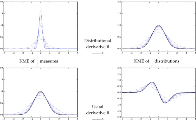
Section1.4first proves the following calculus rules: f, Z k(.,x)dD(x) k = Z hf,k(.,x)_ikdD(x) (Definition of KME) Z k(.,y)dD(y), Z k(.,x)dT(x) k = Z k(x,y)dD(y)d ¯T(x) (Fubini) Z k(.,x)d(∂pS)(x) = (−1)|p| Z ∂(0,p)k(.,x)dS(x). (Differentiation) 17

(34)

While the first two lines extend standard KME formulae, the third one is specific to Schwartz-distributions. It uses the distributional derivative (‘∂’) which extends the usual derivative to measures and distributions (see Appendix A.1). Second, Section 1.4 proves that, for smooth and translation-invariant kernels, extending an injective KME from probability measures to distributions preserves the injec-tivity (Theorems 1.4.5 & 1.4.6). Thus, if the associated MMD is a probability-metric, then it is automatically a metric over these bigger distribution spaces.

The structure of this chapter roughly follows this exposition. After fixing our notations, Section 1.1introduces KMEs of measures and distributions. In Section1.2we define the concepts of universal, char-acteristic and spd kernels and prove their equivalence. Section 1.3 compares convergence in MMD with other modes of convergence for measures and distributions. Section 1.4 focuses specifically on KMEs of Schwartz-distributions, and Section1.5concludes.

Definitions and Notations

The input set X of all considered kernels and functions will be lo-cally compact and Hausdorff. This includes any Euclidian spaces or smooth manifolds, but no infinite-dimensional Banach-space. When-ever referring to differentiable functions or to distributions of order > 1, we will implicitly assume thatX is an open subset of Rd for somed > 0.

A kernel k : X_×X_→ C is a positive definite function, meaning that for all n _∈ N\{0}, all λ1,. . .,λn ∈ C, and all x1,x2,. . .xn ∈

X, Pni,j=1λik(xi,xj)λj > 0. Forp = (p1,p2,. . .,pd) ∈ Nd and f :

X→ C, we define|p|:=Pd_i=1p_iand∂pf:= _∂_p1_x ∂|p|f

1∂p2x2···∂pdxd. For

m_∈N_∪{∞}, we say thatf(resp.k) is m-times (resp.(m,m)-times) continuously differentiable and write f_∈Cm (resp.k_∈C(m,m)), if for any pwith |p|=m,∂pf(resp.∂(p,p)k) exists and is continuous. Cm

b (resp.C m

→0,C m

c ) is the subsets ofCmfor which∂pfis bounded

(resp. converges to0at infinity, resp. has compact support) whenever

|p| ₆ m. Whenever m = 0, we may drop the superscript m. By default, we equip C∗m (∗ ∈ {∅,b,0,c}) with their natural topologies

(see Introduction of [99] or [119]). We write k _∈ C₀(m,m) whenever [99] Simon-Gabriel and Schölkopf, Ker-nel Distribution Embeddings - arXiv, 2016 [119] Treves, Topological Vector Spaces, Distributions and Kernels, 1967

k is bounded, (m,m)-times continuously differentiable and for all

|p|₆mandx_∈X,∂(p,p)k(.,x)_∈C_→₀.

We call space of functionsand denote byFany locally convex (loc. cv.) topological vector space (TVS) of functions (see AppendixA.2). Loc. cv. TVSs include all Banach- or Fréchet-spaces and all function spaces defined in this chapter.

(35)

kernel mean embeddings of distributions | 19

The dualF0of a space of functionsFis the space ofcontinuous lin-ear forms overF. We denoteMδ,Em,Dm_L1 andDm the duals ofCX,

Cm_,_Cm

→0 andCcm respectively. By identifying each signed measure

µwith a linear functional of the formf_7→ Rfdµ, the Riesz-Markov-Kakutani representation theorem (see Appendix A.2) identifies D0

(resp.D0_L1,E0andMδ) with the setMr(resp.Mf,Mc,Mδ) of signed

regular Borel measures (resp. with finite total variation, with com-pact support, with finite support). By definition, D∞ is the set of all Schwartz-distributions, but all duals defined above can be seen as subsets of D∞ and are therefore sets of Schwartz-distributions. Any element µofMr will be called a measure, any element of D∞

a distribution. We extend the usual notationµ(f) :=Rf(x)dµ(x)for measures µ to distributionsD: D(f) =: Rf(x)dD(x). Given a KME Φkand two embeddable distributionsD,T (see Definition1.1.1), we

define

hD,T_ik:=_hΦk(D),Φk(T)ik and kDkk:=kΦk(D)kk .

whereh. , .ikis the inner product of the RKHSHkofk. To avoid

intro-ducing a new name, we call kD_kk the maximum mean discrepancy (MMD) of D, even though the term “discrepancy” usually specifi-cally designates a distance between two distributions rather than the norm of a single one. Given two topological setsS1,S2, we write

S1Continuously Contained inS2

S1,→S2

and say that S1 is continuously contained inS2 if S1 ⊂ S2 and if the

topology of S1 is stronger than the topology induced byS2. For a

general introduction to topology, TVSs and distributions, we

recom-mend [119]. [119] Treves, Topological Vector Spaces, Distributions and Kernels, 1967

1.1

Kernel Mean Embeddings of Distributions

In this section, we show how to embed general distribution spaces into an RKHS. To do so, we redefine the integralRk(.,x)dµ(x)so as to be well-defined even if µis a distribution. It is often defined as a Bochner-integral; here we instead use thePettis- (orweak-) integral:

Definition 1.1.1. Let D be a linear form over a space of functions F. Let ϕ : X_→ Hk be an RKHS-valued function s.t. for any f ∈ Hk, x_{7→ h}f,ϕ(x)_ik _∈ F. Thenϕ : X_→ Hk is weakly integrable with

re-spect to (wrt)Dif there exists a function inHk, written

R

ϕ(x)dD(x), s.t.

Pettis Integral and KME

∀f_∈Hk, f, Z ϕ(x)dD(x) k = Z hf,ϕ(x)_ikd ¯D(x), (1.1)

(36)

where the right-hand-side stands for D¯ (x_{7→ h}f,ϕ(x)_ik)and D¯ denotes the complex-conjugate ofD. Ifϕ(x) =k(.,x), we callRk(.,x)dD(x)the kernel mean embedding (KME) ofDand say thatD embeds intoHk. We

denoteΦϕthe mapΦϕ:D7→

R

ϕ(x)dD(x).

This definition extends the usual Bochner-integral: ifϕis Bochner-integrable wrt a measure µ _∈ Mr, thenϕ is weakly integrable wrt

µ and the integrals coincide [95]. In particular, if x_{7→ k}ϕ(x)_kk is [95] Schwabik,Topics in Banach Space In-tegration, 2005, Prop.2.3.1

Lebesgue-integrable, thenϕis Bochner integrable, thus weakly inte-grable.

The general definition with ϕ instead ofk(.,x) will be useful in Section1.4. But for now, let us concentrate on KMEs whereϕ(x) = k(.,x). Kernels satisfy the so-calledreproducing property: for anyf_∈

Hk, f(x) = hf,k(.,x)ik. Therefore, the condition for all f ∈ Hk x_{7→ h}f,ϕ(x)_ik_∈Freduces toHk⊂F, and Equation (1.1) reads:

Reproducing Property and KMEs ∀f_∈Hk, f, Z k(.,x)dD(x) k =D¯(f). (1.2) Thus, by the Riesz representation theorem (see Appendix A.2), D embeds intoHkiff it defines a continuous linear form overHk. And

in that case, its KME Rk(.,x)dD(x) is the Riesz-representer of ¯D restricted to Hk. Thus, for an embeddable space of distributionsD,

the embeddingΦkcan be decomposed as follows:

Φk:          D −→ H0 k −→ Hk

Conjugate restriction Riesz representer

D _7−→ D¯_H

k 7−→

R

k(.,x)dD(x)

. (1.3)

To know ifDis continuous overHk, we use the following lemma,

and its applications.

Lemma 1.1.2. IfHk,→F, thenF0embeds intoHk.

Proof. Suppose thatHk ,→ F. LetD ∈F0 and letf,f1,f2,. . . ∈Hk.

Iffn →finHk thenfn →f inF, thusD(fn)→D(f). ThusDis a

continuous linear form overHk.

In practice we typically use one of the following two corollar-ies (proofs in Appendices C.1.1 and C.1.2). The space (C_b)c that

they mention will be introduced in the discussions following The-orem 1.2.2. It has the same elements as C_b, but carries a weaker topology.

Corollary 1.1.3. Hk⊂C→0(resp.Hk⊂Cb, resp.Hk⊂C) iff the two

following conditions hold.

Embedding Conditions for Measures (i) For allx_∈X,k(.,x)_∈C_→₀(resp.k(.,x)_∈C_b, resp.k(.,x)_∈C).

(37)

universal, characteristic and SPD kernels | 21

(ii) x_7→ k(x,x)is bounded (resp. bounded, resp.locallybounded, mean-ing that, for eachy_∈X, there exists a (compact) neighborhood ofy

on whichx_7→ k(x,x)is bounded.).

If so, then Hk ,→ C_→0 (resp. Hk ,→ Cb, thus Hk ,→ (Cb)c, resp.

Hk,→C) andMf(resp.Mf, resp.Mc) embeds intoHk.

Corollary 1.1.4.

Embedding Conditions for Distributions Ifk_∈C(m,m), thenHk,→Cm, thusEmembeds intoHk.

Ifk_∈C₀(m,m), thenHk,→C_→m₀, thusDm_L1embeds intoHk.

Ifk_∈C_b(m,m), thenHk,→Cbm, thusHk,→(Cbm)c, thusDmL1 embeds

intoHk.

Corollary1.1.3applied toC_bshows thatHkis (continuously)

con-tained inC_biffkis bounded and separately continuous. As

discov-ered by Lehtö [63], there also exist kernels which are not continuous [63] Lehtö,Some Remarks on the Kernel Function in Hilbert Function Space, 1952

but whose RKHSHkis contained inC_b. So the conditions in

Corol-lary 1.1.4 are sufficient, but in general not necessary. Concerning Lemma 1.1.2, note that it not only requires Hk ⊂ F, but also that

Hkcarries a stronger topology thanF. Otherwise there might exist

a continuous form over F that is defined but non-continuous over

Hk. However, Corollary1.1.3shows that this cannot happen forC∗, because if Hk ⊂ C∗ then Hk ,→ C∗. Although this also holds for

m=∞[99], we do not know whether it extends to anym > 0. [99] Simon-Gabriel and Schölkopf, Ker-nel Distribution Embeddings - arXiv, 2016, Prop.4 & Comments

1.2

Universal, Characteristic and SPD Kernels

The literature distinguishes various variants of universal, character-istic and spd kernels, such as c-, cc− or c0-universal kernels, spd

and integrally strictly positive definite (Rspd) kernels. They are all special cases of the following unifying definitions.

Definition 1.2.1. Letkbe a kernel,Fbe a space of functions s.t.Hk⊂F,

and D be an embeddable subset of F0 (e.g. an embeddable set of distribu-tions). We say thatkis

. universal overFifHkis dense inF.

Universal, Characteristic, SPD . characteristic toDif the KMEΦkis injective overD.

. strictly positive definite (spd) overDif, for allD_∈D,

kΦk(D)k2k=0⇒D=0.

A universal kernel overCm (resp.C_→m₀) will be saidcm- (resp.cm₀ -) uni-versal (without the superscript whenm=0). A characteristic kernel to the setPof probability measures will simply be called characteristic.

kis Characteristic iff its MMD is Perfectly Discriminative onP Importantly, note that k is characteristic to P iff the MMD of k

(38)

k is characteristic hence amounts to determining when the associ-ated MMD is perfectly discriminative. In general, instead of writing

kΦk(D)kk andhΦk(D),Φk(T)ik, we will writekDkk andhD,Tik.

The previous definitions encompass the usual spd definitions. Denot-ingδxthe Dirac measure concentrated onx, what is usually called

. spd corresponds toD=Mδ, i.e. ∀µ= n X i=1 λiδxi ∈Mδ:        kµ_k2_k= n X i,j=1 λik(xi,xj)λ¯j=0 =_⇒ λ1=. . .=λn=0. Specific SPD Instances . conditionally spd corresponds toD = M0_δ whereM0_δ :={µ _∈

Mδ:µ(X) =0}, i.e.: ∀µ=Xn i=1λiδxi ∈Mδ s.t. Xn i=1λi=0: kµ_k2_k= n X i,j=1 λik(xi,xj)λ¯j=0 =⇒ λ1=. . .=λn=0. . Rspd corresponds toD=Mf, i.e. : ∀µ_∈Mf: kµk2k= ZZ k(x,y)dµ(x)d ¯µ(y) =0 _⇒ µ=0. Let us now state the general link between universal, characteristic and spd kernels, which is the key that underlies Figure 1 in [109].

[109] Sriperumbudur et al.,Universality, Characteristic Kernels and RKHS Embed-ding of Measures, 2011

Theorem 1.2.2. IfHk,→F, then the following statements are equivalent.

Equivalence of Universality, Characteristicness and SPD (i) kis universal overF.

(ii) kis characteristic toF0.

(iii) kis strictly positive definite (spd) overF0.

Proof. Equivalence of(ii)&(iii): Saying thatkΦk(D)kk=0is

equiv-alent to sayingΦk(D) = 0. Thus Φk is spd overF0 iff the Ker(Φk)

(meaning the vector space that is mapped to0viaΦ_k) is reduced to

{0}, which happens iffΦ_kis injective overF0.

Equivalence of (i) & (ii): Φ_k is the conjugate restriction opera-tor |_H_k : D_7→ D¯|_H

k composed with the Riesz representer mapping

(Diagram Eq.1.3). The Riesz representer map is injective, so Φ_k is injective iff |_H_k is injective. Now, ifHk is dense inF, then, by

con-tinuity, any D _∈ F0 is uniquely defined by its values taken onHk.

Thus|_Hk is injective. Reciprocally, ifHkis not dense inF, then, by

the Hahn-Banach theorem [119], there exists two different elements [119] Treves, Topological Vector Spaces, Distributions and Kernels, 1967, Thm.18.1, Cor.3

inF0that coincide onHkbut not on the entire spaceF. So|_Hk is not

injective. Thus|Hk is injective iffHkis dense inF.

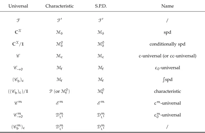
To apply this theorem it suffices to find so-called duality pairs (F,F0) s.t.Hk ,→ F. Table 1.1lists several such pairs. It shows in

(39)

universal, characteristic and SPD kernels | 23

Universal Characteristic S.P.D. Name

F F0 _F0 _/

CX Mδ Mδ spd

CX/₁ M0_δ M0_δ conditionally spd

C Mc Mc c-universal (orcc-universal)

C→0 Mf Mf c0-universal (C_b)c Mf Mf R spd ((C_b)c)/1 P(orMf0) Mf0 characteristic Cm _Em _Em _cm_-universal Cm →0 DmL1 D m L1 c m 0 -universal (C_bm)c Dm_L1 Dm_L1 /

Table 1.1: Equivalence between the no-tions of universal, characteristic and spd kernels as implied by Thm.1.2.2or Prop.1.2.3.

particular the well-known equivalence betweenc- (resp.c₀-) univer-sal kernels and characteristic kernels toMc(resp.Mf) [110]. But we

[110] Sriperumbudur et al., Injective Hilbert Space Embeddings of Probability Measures, 2008

now discover that spd kernels over Mδ can also be characterized in

terms of universality over CX, because (CX)0 = M_δ [26]. And we

[26] Duc-Jacquet, Approximation des Fonctionnelles Linéaires sur les Espaces Hilbertiens Autoreproduisants, 1973, p.II.35

directly get the generalization to distributions andcm_∗ -universality. However, Theorem 1.2.2leaves open the important case where k is characteristic (to P). Of course, asPis contained in Mf, it shows

that ac0-universal kernel must be characteristic. But to really

charac-terize characteristic kernels in terms of universality, we would need to find a predual ofP, meaning a spaceFs.t.F0=P. This is hardly possible, asPis not even a vector space. However, we will see in The-orem 1.2.4that kis characteristic iffk is characteristic to the vector spaceMf0:={µ∈Mf:µ(X) =0}. So if we find a predual ofMf0, then

we get an analog of Theorem1.2.2applied toP. Let us do so now.

Predual ofPandM0 f?

As Mf0 is the hyperplane of Mf that is given by the equation

R

1dµ=0, our idea is to take a predualFofMfand consider the

quo-tient F/₁of Fdivided by the constant function 1. Proposition 35.5

of [119] would then show that (F/₁)0 = M_f0. But if we take the [119] Treves, Topological Vector Spaces, Distributions and Kernels, 1967

usual predual of Mf, F = C_→0, then 1 6∈ F, so the quotient F/1

is undefined. However, preduals are not unique, so let us try with another space F that contains 1, for example F = C_b. This time 1 ∈ F, but now the problem is that F0 is in general strictly bigger

than Mf [28] whereas we want F0 = Mf. The trick now is to keep [28] Fremlin et al.,Bounded Measures on

Topological Spaces, 1972, Sec.2 §2

(40)

F0_{becomes smaller. Intuitively, the reason for this decrease of}_F0 _is that, by weakening the topology of F, we let more sequences con-verge in F. This makes it more difficult for a functional overF to be continuous, because for any converging sequence inF, its images need to converge. Thus some of the linear functionals that were con-tinuous for the original topology ofF get “kicked out” ofF0when

Fcarries a weaker topology. Now the only remaining step is to find a topology s.t. that F0 shrinks exactly toMf. There are at least two

such topologies: one defined by [96] and another, called the strict

[96] Schwartz, Espaces de fonctions dif-férentiables à valeurs vectorielles, 1954, p.100-101

topology, whose definition can be found in [28]. Denotingτc either

[28] Fremlin et al.,Bounded Measures on Topological Spaces, 1972

of these topologies, and (C_b)c the space C_b equipped with τc, we

finally get((C_b)c)0=Mf, and thus:

Universal-Characteristic Equivalence forP Proposition 1.2.3. ((C_b)c/1)0 =M_f0. Thus, ifHk ,→(Cb)c, thenkis

characteristic toPiffkis universal over the quotient space((C_b)c/1).

Proof. That((C_b)c)0=Mfis proven in [28] or [96]. Prop. 35.5 of [119]

[28] Fremlin et al.,Bounded Measures on Topological Spaces, 1972, Thm.1

[96] Schwartz, Espaces de fonctions dif-férentiables à valeurs vectorielles, 1954, p.100-101

[119] Treves, Topological Vector Spaces, Distributions and Kernels, 1967

then implies((C_b)c/1)0 =M_f0(becauseM_f0 is the so-calledpolar set

of1; see [119]). Thm1.2.2implies the rest.

For our purposes, the exact definition ofτcdoes not matter. What

matters more is that τcis weaker than the usual topology ofCb, so

that if Hk ,→Cb, thenHk ,→ (Cb)c. Proposition 1.2.3thus applies

every time thatHk⊂Cb (see Corollaries 1.1.3and 1.1.4). However,

we do not know of any practical application of Proposition 1.2.3, except that it completes our overall picture of the equivalences be-tween universal, characteristic and spd kernels. Let us also mention that, similarly to Proposition 1.2.3, as (CX)0 = Mδ, we also have

(CX/₁)0=M0_δ. So conditionally spd kernels (meaning spd overM0 δ)

are universal toCX/₁.

We now prove what we announced and used earlier: a kernel is characteristic to P iff it is characteristic to M0

f. We add a few

other characterizations which are probably more useful in practice. They rely on the following observation: asM0

f is a hyperplane ofMf,

saying thatkis characteristic toPis almost the same as saying that it is characteristic toMf, i.e.

R

spd (Thm.1.2.2): after all, there is only one dimension needed to go fromM0

f toMf. Thus there should be a

way to construct anRspd kernel out of any characteristic kernel. This is what is described here and proven in AppendixC.1.3.

Theorem 1.2.4. Letk0be a kernel. The following is equivalent.

From Characteristic toRSPD Kernels and Back (i) k0is characteristic toP.

(ii) k0is characteristic toMf0.

(iii) There exists_∈Rs.t. the kernelk(x,y) :=k0(x,y) +2is

R spd. (iv) For all_∈R\{0}, the kernelk(x,y) :=k0(x,y) +2is

R spd. (v) There exists an RKHSHkwith kernelkand a measureν0∈Mf\Mf0

(41)

topology induced by k | 25

Under these conditions, k0 and k induce the same MMD semi-metric in

M0

f and inP.

We will use this theorem to prove Theorem 1.3.4. Intuitively, a characteristic kernel guarantees that two signed measures µ1,µ2

with same total mass get mapped to two different functions in the RKHS. This is captured by (ii)which arbitrarily focuses on the spe-cial case where the total mass is 0. When they have different total masses however, they may get mapped to a same function f, except if, like in (iii)and (iv), we add a positive constant to the kernel. In that case, µ1 and µ2 get mapped to the functions f+µ1(X)1 and

f+µ2(X)1 which are now different, becauseµ1(X) 6= µ2(X).

Intu-itively, by adding a positive constant to our kernel, we added one dimension to the RKHS (carried by the function 1) that explicitly ‘checks’ if two measures have the same mass. Finally,(v)tells us that, out of anyRspd kernelk, we can construct a characteristic kernelk0

that is notRspd anymore and vice-versa.

1.3

Topology Induced by

k

Remember that for any distribution D of a set of embeddable dis-tributions D we defined kD_kk := _kΦ_k(D)_kk and called kD_kk the maximum mean discrepancy (MMD) ofD. Doing this defines a new topology on D, in which a net Dα converges to D iff kDα−Dkk

converges to0. (A reader unfamiliar with nets may think of them as

sequences where the indexαcan be continuous; see [9].) In this sec- [9] Berg et al., Harmonic Analysis on Semigroups Theory of Positive Definite and Related Functions, 1984

tion, we investigate how convergence in MMD compares with other types of convergences defined onDthat we now shortly present.

We defined Das a subset of a dual spaceF0, soD will carry the topology induced by F0. Many topologies can be defined on dual spaces, but the two most prominent ones, which we will consider here, are the weak-∗ and the strongtopology, denoted w(F0,F)and b(F0,F) respectively, or simplyw_∗ and b. The weak-∗ topology is

Convergences on Dual Spaces: Weak-∗and Strong Convergence the topology of pointwise convergence (where by ‘point’, we mean a

function inF), while the strong topology corresponds to the uniform convergence over the bounded subsets of F(see Eq. 1.2). Bounded sets of a TVS are defined in AppendixA.2(DefinitionA.2.4). By de-fault, we equipF0with the strong topology and sometimes writeFb0

to emphasize it. WhenFis a Banach space, the strong topology ofF0 is the topology of the operator norm kD_k_F0 :=sup_k_f_k

F61|D(f)|. In particular, strong convergence in Mf = (C→0)0 means convergence

in total variation (TV) norm and weak-_∗ convergence inMf means

convergence for any functionf_∈C_→₀. OnMf, we will also consider

the topology of pointwise convergence overC_b (instead ofC_→₀). It is widely used in probability theory where it is known as theweak(or

(42)

narrow) convergence topology. We will denote it byσ. Importantly, Weak-∗Convergence Coincides with Weak Convergence onP the weak and weak-∗topologies ofMf coincide onP(but not onMf)

[9]. Finally, we define the weak RKHS convergence of embeddable

[9] Berg et al., Harmonic Analysis on Semigroups Theory of Positive Definite and Related Functi