Side Information in Robust Principal Component Analysis: Algorithms and
Applications
Niannan Xue
Imperial College London, UK
[email protected]Yannis Panagakis
Imperial College London, UK
Middlesex University, UK
[email protected]Stefanos Zafeiriou
Imperial College London, UK
Abstract
Robust Principal Component Analysis (RPCA) aims at recovering a low-rank subspace from grossly corrupted high-dimensional (often visual) data and is a cornerstone in many machine learning and computer vision applications. Even though RPCA has been shown to be very success-ful in solving many rank minimisation problems, there are still cases where degenerate or suboptimal solutions are ob-tained. This is likely to be remedied by taking into account of domain-dependent prior knowledge. In this paper, we propose two models for the RPCA problem with the aid of side information on the low-rank structure of the data. The versatility of the proposed methods is demonstrated by ap-plying them to four applications, namely background sub-traction, facial image denoising, face and facial expression recognition. Experimental results on synthetic and five real world datasets indicate the robustness and effectiveness of the proposed methods on these application domains, largely outperforming six previous approaches.
1. Introduction
Principal Component Pursuit (PCP) as proposed in [7,8] and its variants e.g. [2, 3, 5, 25, 33, 36] are the current methods of choice for recovering a low-rank subspace from a set of grossly corrupted and possibly incomplete high-dimensional data. PCP employs the nuclear norm and the l1 norm (convex surrogates of the rank and sparsity con-straints, respectively) in order to approximate the original l0norm regularised rank minimisation problem. In particu-lar, under certain conditions (such as the restricted isometry property [6]), the relaxation gap is zero and rank minimisa-tion is equivalent to nuclear norm minimisaminimisa-tion. However, these conditions rarely hold for real-world visual data and PCP thus occasionally yields degenerate or suboptimal so-∗The work of Stefanos Zafeiriou was partially funded by EPSRC project EP/N007743/1 (FACER2VM).
lutions. To alleviate this, it is advantageous for PCP to take into account of domain-dependent prior knowledge [13], i.e. side information [32].
The use of side information has been studied in the con-text of matrix completion [9,34] and compressed sensing [17]. Recently, side information has been applied to the PCP framework in thenoiselesscase [10,21]. In particu-lar, an error-free orthogonal column space was used to drive a PCP-based deformable image alignment algorithm [21]. More generally, Chianget al. [10] used both a column and a row space as side information and the algorithm had to re-cover the weights of their interaction. The main limitation of such methods is that they require a set of clean, noise-free data samples in order to determine the column and/or row spaces of the low-rank component. Clearly, these data are are difficult to find in practice.
In this paper, we investigate the idea of using a noisy approximation of the low-rank component to guide PCP. Knowledge regarding the low-rank component, albeit noisy, is available in many applications. In background subtrac-tion, we may find some frames of the video that do not con-tain changes and therefore may be used to accurately esti-mate the background. Another example concerns the prob-lem of disentangling identity and expression components in expressive faces, where the low-rank component is roughly similar to the neutral face. Note that side information which has the same form as the source is already subject to wide-spread usage. Watermark detection methods require a ref-erence image to identify ownership [11]. Automated photo tagging explores visually similar social images [31]. Lo-cality preserving projection can be enhanced by exploiting similar pairs of patterns [1]. Spatial and temporal correla-tion can improve signal recovery algorithms in compressive imaging [26]. In content-based image retrieval, historical feedback log data can help retrieve semantically relevant images [35]. Low-resolution images can help adapt a high-resolution compressive sensing system [29]. Near-accurate fingerprint or DNA can be used as side information to hack a biometric authentication system [14].
Our contributions are summarised as follows:
• A novel convex program is proposed to use side in-formation, which is a noisy approximation of the low-rank component, within the PCP framework with a provably convergent solver.
• Furthermore, we extend our proposed PCP model us-ing side information to exploit prior knowledge regard-ing the column and row spaces of the low-rank compo-nent in a more general algorithmic framework.
• We demonstrate the applicability and effectiveness of the proposed approaches in several applications, namely background subtraction, facial image denois-ing as well as face recognition and facial expression classification.
• We also show that our proposed methods can mitigate the transductive constraint of RPCA. With side infor-mation, training can be performed on fewer samples and hence reducing the computational cost.
NotationsLowercase letters denote scalars and uppercase
letters denote matrices, unless otherwise stated. For norms of matrix A, kAkF is the Frobenius norm; kAk∗ is the nuclear norm; and kAk∞is the maximum absolute value among all matrix entries. Moreover, hA,Bi represents tr(ATB) for real matricesA,B. Additionally,σ
iis theith
largest singular value of a matrix andσj% is the singular value at thejth percentile.
2. Related work
The problem of incorporating side information in esti-mating low-rank components can be stated as follows. Sup-pose that there is a matrix L0 ∈ Rn1×n2 with rank r ≪ min(n1, n2) and a sparse matrixS0 ∈Rn1×n2 with entries of arbitrary magnitude. If we are provided with the data matrix
M=L0+S0, (1)
and additional side information, how can we recover the low-rank componentL0and the sparse noiseS0accurately by taking advantage of the side information?
One the first methods for incorporating side information was proposed in the context of deformable face alignment [21]. The RAPS algorithm assumes that we have available an orthogonal column spaceX∈Rn1×d1, whered1≤n1,
and
minimise
G,S kGk∗+λkSk1
subject to XG+S=M. (2)
A generalisation of the above was proposed as Principal Component Pursuit with Features (PCPF) in [10] where fur-ther row spacesY∈Rn2×d2were assumed to be available
withd2≤n2, and minimise
H,S kHk∗+λkSk1 subject to XHYT +S=M.
(3)
Shahidet al. [23,24] incorporate structural knowledge into RPCA by adding spectral graph regularisation. Given the graph Laplacian Φof each data similarity graph, Ro-bust PCA on Graphs (RPCAG) and Fast RoRo-bust PCA on Graphs (FRPCAG) add an additional tr(LΦLT)
term to the PCP objective for the low-rank component L. The main drawback of the above mentioned models is that the side in-formation needs to be accurate and noiseless, which is not trivial in practical scenarios.
3. Robust Principal Component Analysis Using
Side Information
In this section, the proposed RPCA models with side formation are introduced. In particular, we propose to in-corporate the side information into PCP by using the trace distance of the difference between the low-rank component and the noisy estimate, which is reasonable if their differ-ence is of low rank. However, we show empirically (Section
4) that it also works if the difference is full-rank. This may be attributed to the fact that the trace distance is a natural distance metric between two dissimilar distributions from Kolmogorov−Smirnov statistics [18]. Besides that, this is a generalisation of the compressed sensing with side infor-mation where thel1norm has been used in order to measure the distance of the target signal with prior information [17].
3.1. The PCPS model
Assuming that a noisy estimate of the low-rank compo-nent of the dataW∈Rn1×n2 is available, we propose the
following model of PCP using side information (PCPS): minimise
L,S kLk∗+κkL−Wk∗+λkSk1 subject to L+S=M,
(4)
whereκ > 0, λ >0are parameters that weigh the effects of side information and noise sparsity.
The proposed PCPS can be revamped to generalise the previous attempt of PCPF by the following objective of PCPS with features (PCPSF):
minimise
H,S kHk∗+κkH−Dk∗+λkSk1 subject to XHYT +S=M, XWYT =D,
(5)
whereH ∈ Rd1×d2,D ∈ Rd1×d2 are bilinear mappings
for the recovered low-rank matrix Land side information
W respectively. If W = L+C, then D = XT(L+
onto a smaller region Rd×d
rather than Rn×n
which has made the problem easier to solve. Note that the low-rank matrixL is recovered from the optimal solution (H∗,S∗) to objective (5) viaL =XH∗YT. If side informationW
is not available, PCPSF reduces to PCPF by setting κto zero. If the featuresX,Yare not present either, PCP can be restored by fixing both of them at identity. However, when only the side informationWis accessible, objective (5) is transformed back into PCPS.
3.2. The algorithm
If we substituteEforH−Dand orthogonaliseXand
Y, the optimisation problem (5) is identical to the following convex but non-smooth problem:
minimise
H,S kHk∗+κkEk∗+λkSk1
subject to XHYT +S=M, E−H=−XTWY, (6)
which is amenable to the multi-block alternating direction method of multipliers (ADMM).
The corresponding augmented Lagrangian of (6) is: l(H,E,S,Z,N) =kHk∗+κkEk∗+λkSk1 +hZ,M−S−XHYTi+µ 2kM−S−XHY Tk2 F +hN,H−E−XTWYi+µ 2kH−E−X TWYk2 F, (7)
whereZ ∈ Rn1×n2 andN ∈ Rd1×d2 are Lagrange
multi-pliers andµis the learning rate.
The ADMM operates by carrying out repeated cycles of updates till convergence. During each cycle, H,E,S
are updated serially by minimising (7) with other variables fixed. Afterwards, Lagrange multipliersZ,Nare updated at the end of each iteration. Direct solutions to the sin-gle variable minimisation subproblems rely on the shrink-age and the singular value thresholding operators [7]. Let
Sτ(a)≡sgn(a) max(|a| −τ,0)serve as the shrinkage
op-erator, which naturally extends to matrices,Sτ(A), by
ap-plying it to matrixAelement-wise. Similarly, letDτ(A)≡
USτ(Σ)VT be the singular value thresholding operator on
real matrixA, withA =UΣVT being the singular value
decomposition (SVD) ofA.
Minimising (7) w.r.t.Hat fixedE,S,Z,Nis equivalent to the following: arg min H kHk∗+µkP−XHY Tk2 F, (8) whereP= 1 2(M−S+W+ 1 µZ+X(E− 1 µN)Y T). Its solution is shown to beXTD 1 2µ (P)Y. Furthermore, forE, arg min E l= arg minE κkEk∗+ µ 2kQ−Ek 2 F, (9)
Algorithm 1ADMM solver for PCPSF
Input: Observation M, side information W, features
X,Y, parametersκ, λ >0, scaling ratioα >1. 1: Initialize:Z= 0,N=E=H= 0,µ= kM1k
2.
2: whilenot convergeddo 3: S=Sλµ−1(M−XHYT + 1 µZ) 4: H = XTD1 2µ( 1 2(M −S+W + 1 µZ +X(E− 1 µN)Y T))Y 5: E=Dκµ−1(H−X TWY+1 µN) 6: Z=Z+µ(M−S−XHYT) 7: N=N+µ(H−E−XTWY) 8: µ=µ×α 9: end while Return: L=XHYT,S whereQ = H−XTWY+ 1
µN, whose update rule is
Dκ µ(Q), and forS, arg min S l= arg minS λkSk1+ µ 2kR−Sk 2 F, (10)
whereR=M−XHYT +µ1Zwith a closed-form solu-tionSλµ−1(R). Finally, Lagrange multipliers are updated
as usual:
Z=Z+µ(M−S−XHYT), (11)
N=N+µ(H−E−XTWY). (12) The overall algorithm is summarised in Algorithm1.
3.3. Complexity and convergence
Orthogonalisation of the features X,Y via the Gram-Schmidt process has an operation count of O(n1d21) and O(n2d22)respectively. TheHupdate in Step4is the most costly step of each iteration in Algorithm 1. Specifically, the SVD required in the singular value thresholding action dominates withO(min(n1n2
2, n2
1n2))complexity.
It has been recently established that for a 3-block sepa-rable convex minimisation problem, the direct extension of the ADMM achieves global convergence with linear con-vergence rate if one block in the objective is sub-strongly monotonic [27]. In our case, it can be shown thatkSk1 processes such sub-strong monotonicity. We have also used the fast continuation technique to increaseµincrementally for accelerated superlinear performance. The cold start initialisation strategies for variables H,E and Lagrange multipliers Z,N are described in [4]. Besides, we have scheduled Sto be updated first. As for stopping criteria, we have employed the Karush-Kuhn-Tucker (KKT) fea-sibility conditions. Namely, within a maximum number of 1000 iterations, when the maximum of kM − Sk −
dwindles from a pre-defined thresholdǫ, the algorithm is terminated, whereksignifies values at thekth
iteration.
4. Experimental results
In this section, we illustrate the enhancement made by side information through both numerical simulations and real-world applications. First, we compare the recoverabil-ity of our proposed algorithms with state-of-the-art meth-ods for incorporating features or dictionaries,i.e. PCPF [10] and RAPS [21] on synthetic data as well as the baseline PCP [7] when there are no features available. Second, we show how powerful side information can be for the task of object segmentation in video pre-processing. Third, we demonstrate that side information is instructive in the low-dimensionality face modeling from images of different illu-minations. Last, we reveal that the more accurately recon-structed expressions in the light of side information lead to better emotion classification.
For RAPS, clean subspaceXis used instead of the ob-servation Mitself as the dictionary in LRR [15]. PCP is solved via the inexact ALM and the heuristics for predict-ing the dimension of principal spredict-ingular space is not adopted here due to its lack of validity on uncharted real data. We also include Partial Sum of Singular Values (PSSV) [19] in our comparison for its stated advantage in view of the lim-ited number of expression observations available.
4.1. Parameter calibration
The process of tuning the algorithmic parameters for various models is described in the supplementary mate-rial. Although theoretical determination ofκandλis be-yond the scope of this paper, we nevertheless provide em-pirical guidance based on extensive experiments. λ = 1/pmax(n1, n2)for a general matrix of dimensionn1×n2 from PCP works well for both of our proposed models. κ depends on the quality of the side information. When the side information is accurate, a large κshould be selected to capitalise upon the side information as much as possible, whereas when the side information is improper, a smallκ should be picked to sidestep the dissonance caused by the side information. Here, we have discovered that aκvalue of0.2works best with synthetic data and a value of0.5is suited for public video sequences. It is worth emphasis-ing again that prior knowledge of the structural information about the data yields more appropriate values forκandλ.
4.2. Phase transition on synthetic datasets
We now focus on the recoverability problem,i.e. recov-ering matrices of varying ranks from errors of varying spar-sity. True low-rank matrices are created via L0 = JKT, where200×r matricesJ,K have independent elements drawn randomly from a Gaussian distribution of mean 0
and variance5·10−3
soris the rank ofL0. Next, we gen-erate200×200error matricesS0, which possessρs·2002
non-zero elements located randomly within the matrix. We consider two types of entries for S0: Bernoulli ±1 and
PΩ(sgn(L0)), whereP is the projection operator andΩis the support set ofS0.M=L0+S0thus becomes the sim-ulated observation. For each(r, ρs)pair, three observations
are constructed. The recovery is successful if for all these three problems,
kL−L0kF
kL0kF
<10−3 (13)
from the recoveredL. In addition, letL0 = UΣVT be the SVD of L0. FeatureX is formed by randomly inter-weaving column vectors ofUwithdarbitrary orthonormal bases for the null space of UT, while permuting the ex-panded columns ofVwithdrandom orthonormal bases for the kernel of VT
forms feature Y. Hence, the feasibility conditions are fulfilled: C(X)⊇C(L0),C(Y)⊇C(LT0), whereCis the column space operator.
Entry-wise corruptions. For these trials, we construct the side information by directly adding small Gaussian noise to each element ofL0:lij→lij+N(0,2.5r·10−9),
i, j = 1,2,· · ·,200. As a result, the standard deviation of the error in each element is 1%of that among the ele-ments themselves. On average, the Frobenius percent error,
kW−L0kF/kL0kF, is1%. Such side information is
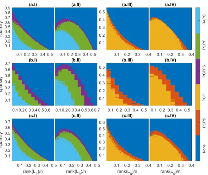
gen-uine in regard to the fact that classical PCA with accurate rank is not able to eliminate the noise [22]. For d = 10, Figures1(a.I) and1(a.II) plot results from PCPF, RAPS and PCPSF. On the other hand, the situation with no available features is investigated in Figures 1(a.III) and 1(a.IV) for PCP and PCPS. The frontier of PCPF has been advanced by PCPSF everywhere for both sign types. Especially at low ranks, errors with much higher density can be removed. Without features, PCPS surpasses PCP by and large with significant expansion at small sparsity for both cases.
Deficient ranks. Now we first make a new matrix Σ′
by retaining only the singular values fromσ1toσ90%inΣ. Then, side information is constructed according to W = UΣ′VT, aka hard thresholding. As rank increases,
Frobe-nius percent error ofWdecreases from23.3%to5.8% sub-linearly. Figures1(b.I) and1(b.II) show results from PCPF, RAPS and PCPSF where dis again kept at10. The cor-responding cases with no features are presented in Figures
1(b.III) and1(b.IV) for PCP and PCPS. Notwithstanding the most spurious side information, PCPSF and PCPS have re-claimed the largest region unattainable by PCPF and PCP respectively for the two signs.
Distorted singular values. Here, we produce the ma-trixΣ′ by adding Gaussian noise to singular values inΣ: σi→σi+ 0.01· N(0, σ
2
i)for alli. Next, side information
Figure 1: Domains of recovery by various algorithms: (I,III)for random signs and (II,IV)for coherent signs. (a) for entry-wise corruptions,(b)for deficient ranks and(c)for distorted singular values.
error inWis1%. Withdrelaxed to50, recoverability dia-grams for PCPF, RAPS, PCPSF and PCP, PCPS are drawn in Figures (c.I), (c.II) and (c.III), (c.IV). We observe sub-stantial growth of recoverability for PCPS over PCP across the full range of ranks. And with features, there is still omniscient gain in recoverablity for PCPSF against PCPF, which is marked at low ranks.
We remark that in unrecoverable areas, PCPS and PCPSF still obtain much smaller values of kL−L0kF.
In view of the marginal improvement of RAPS contrasted with PCPF and PCPSF, we will not consider it any longer. Results from RPCAG and PSSV are worse than PCP (see the supplementary material). FRPCAG fails to recover any-thing at all.
4.3. Face denoising under variable illumination
It has been previously proved that a convex Lambertian surface under distant and isotropic lighting has an underly-ing model that spans a 9-D linear subspace. Albeit faces can
be described as Lambertian, it is only approximate and har-monic planes are not real images due to negative pixels. In addition, theoretical lighting conditions cannot be realised and there are unavoidable occlusion and albedo variations. It is thus more natural to decompose facial image formation as a low-rank component for face description and a sparse component for defects. What is more, we suggest that fur-ther boost to the performance of facial characterisation can be gained by leveraging an image which faithfully repre-sents the subject.
We consider images of a fixed pose under different il-luminations from the extended Yale B database for testing. Ten subjects were randomly chosen and all 64 images were studied for each person. For single-person experiments, 32556×64observation matrices were formed by vectorising each168×192image and the side information was chosen to be the average of all images, tiled to the same size as the observation matrix for each subject. For the multiperson ex-periment, both single-person observation and side
informa-(a) (b) (c) (d) (e) (f) (g) (h) (i)
Figure 2: Comparison of face denoising ability: In row I,(a, e)sample frames from subjects 2 and 33;(b, f)single-person PCP;(c, g)single-person PCPF;(h, i)multi-person PCP and PCPF;(d)average of other subjects. In row II,(a, e)average of a single subject;(b, f)single-person PCPS;(c, g)single-person PCPSF;(h, i)multi-person PCPS and PCPSF;(d)PCPS using the side information above.
tion matrices were concatenated into32556×640matrices respectively.
For PCPF and PCPSF to run, we learn the feature dictio-nary following an approach by Vishalet al. [20]. In a nut-shell, the feature learning process can be treated as a sparse encoding problem. More specifically, we simultaneously seek a dictionaryD ∈ Rn1×c and a sparse representation B∈Rc×n2 such that: minimise D,B kM−DBk 2 F subject to γi≤tfori= 1. . . n2, (14)
wherecis the number of atoms,γi’s count the number of
non-zero elements in each sparsity code andt is the spar-sity constraint factor. This can be solved by the K-SVD algorithm. Here, featureXis the dictionaryD, featureY
corresponds to a similar solution using the transpose of the observation matrix as input and the sparse codes are
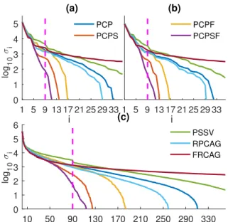
irrel-1 5 9 irrel-13 irrel-17 2irrel-1 25 29 33 i 0 1 2 3 4 5 log 1 0 σ i (a) PCP PCPS 1 5 9 13 17 21 25 29 33 i (b) PCPF PCPSF 10 50 90 130 170 210 250 290 330 i 0 1 2 3 4 5 6 log 1 0 σ i (c) PSSV RPCAG FRCAG
Figure 3: Log-scale singular values of the denoised matri-ces:(a)subject 2;(b)subject 33;(c)all subjects.
evant. For implementation details, we set cto40,tto40 and used10iterations. Because K-SVD could not converge in reasonable time for the multiperson experiment, we re-sorted to classical PCA applied to the observation matrix to obtain featuresX,Yof dimension400.
As a visual illustration, two challenging cases are exhib-ited in Figure2(PSSV, RPCAG, FRPCAG do not improve upon PCP and are shown in the supplementary material). For subject 2, it is clearly evident that PCPS and PCPSF outperform the best existing methods through the complete elimination of acquisition faults. More surprisingly, PCPSF even manages to restore the flash in the pupils that is not present in the side information. For subject 33, PCPS in-dubitably reconstructs a more vivid left eye than that from PCP which is only discernible. With that said, PCPSF still prevails by uncovering more shadows, especially around the medial canthus of the left eye, and revealing a more distinct crease in the upper eyelid as well a more translucent iris. We also notice that results from the single-person experiment outdo their counterparts from the multiperson experiment. Thence, we will focus on a single subject alone.
To quantitatively verify the improvement made by our proposed approaches, we examine the structural informa-tion contained within the deionised eigenfaces. Singular values of the recovered low-rank matrices from all algo-rithms are plotted in Figure3. Singular values decease most sharply for PCPSF followed by PCPS. By the theoretical limit, they are orders of magnitude smaller than those val-ues from other methods. This validates our proposed ap-proaches.
We further unmask the strength of PCPS by considering the stringent side information made of the average of other subjects. Surprisingly, PCPS still manages to remove the noise recovering an authentic image (see Figure2(d)).
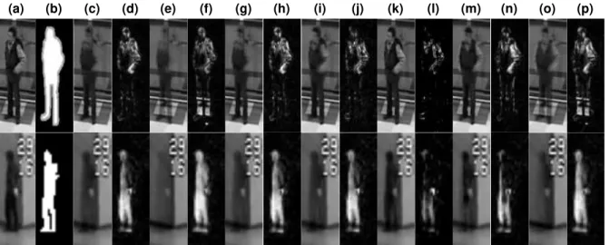
(a) (b) (c) (d) (e) (f) (g) (h) (i) (j) (k) (l) (m) (n) (o) (p)
Figure 4: Background subtraction results for two sample frames, PETS in row I and Airport in row II:(a)original images;
(b)ground truth;(c,d)PCP;(e,f)PCPS;(g,h)PSSV;(i,j)RPCAG;(k,l )FRPCAG;(m,n)PCP (60 frames);(o,p)PCPS (60 frames).
4.4. Background subtraction from surveillance
video
In automated video analytics, object detection is in-strumental in object tracking, activity recognition and behaviour understanding. Practical applications include surveillance, traffic control, robotic operation, etc., where foreground objects can be people, vehicles, products and so forth. Background subtraction segments moving objects by calculating the pixel-wise difference between each video frame and the background. For a static camera, the back-ground is almost static, while the foreback-ground objects are mostly moving. Consequently, a decomposition into a low-rank component for the background and a sparse compo-nent for foreground objects is a valid model for such dy-namics. Indeed, if the only change in the background is illumination, then the matrix representation of vectorised backgrounds has a rank of1. It has been demonstrated that PCP is quite effective for such a low-rank matrix analysis problem [7]. Nevertheless, through the application of our proposed algorithm to such a background-foreground sep-aration scenario, we show that useful side information can
10 50 90 130 170 Frame 0 0.05 0.1 0.15 0.2 0.25 0.3 Weighted F-measure (a) PCP PCPS 1 2 3 4 5 6 7 8 9 Frame 0.2 0.25 0.3 0.35 0.4 0.45 (b) PSSV RPCAG FRPCAG
Figure 5: Weighted F-measure scores: (a)PETS;(b) Air-port.
help achieve better background restoration.
One video sequence from the PETS 2006 dataset and one from the I2R dataset were utilised for evaluation. Each con-sists of scenes at a hall where people walk intermittently. 200 consecutive frames of720×576resolution grayscale images were stacked by columns into a414720×200 ob-servation matrix from the first video and 200 frames of 176×144images from the second video were stacked into another25344×200observation matrix. Two side infor-mation arrays comprised columns that are copies of a vec-torised photo which contains an empty hallway. To com-mence object detection, PCP and PCPS were first run to extract the backgrounds. Then objects were recovered by calculating the absolute values of the difference between the original frame and the estimated background. Since param-eters for dictionary learning need exhaustive search, we will not be comparing PCPF and PCPSF for what follows.
We quantitatively compare the performance of the com-peting methods according to the weighted F-measure [16] against manually annotated bounding boxes provided as the ground truth. The resulting scores for each frame are pre-sented in Figure5. From the consistently higher precision statistics, the merit of PCPS over PCP is confirmed. For qualitative reference, representative images of the recov-ered background and foreground from all methods are listed in Figure4 (For space reasons, we have only included the most noticeable sector. See the supplementary material for whole images.). PCP and its variants only partially detect infrequent moving objects, people who stop moving for ex-tended periods of time, leaving ghost artifacts in the back-ground. In contrast, PCPS segments a fairly sharp silhouette of slowly moving objects to produce a much cleaner back-ground, promoting its novelty.
shortened videos from PETS and Airport consisting of 60 frames are analysed via PCPS. Figures4(c,d)&(o,p)show that PCPS with less input can achieve comparative or bet-ter results than PCP with more input. This suggests that the transductive constraint of RPCA no longer applies because with the help of side information we can run PCPS on fewer frames rather than the entire collection every time new ob-servation arrives. The speed-ups for PETS and Airport are 2.44×and2.62×respectively.
4.5. Face and facial expression recognition
Recent research has established that an expressive face can be treated as a neutral face plus a sparse expression component [28], which is identity-independent due to its constituent local non-rigid motions,i.e. action units. This is central to computer vision as it enables human emotion clas-sification from such visual cues. We will demonstrate how the accurate reconstruction of facial expressions guided by side information ameliorates classification analysis.
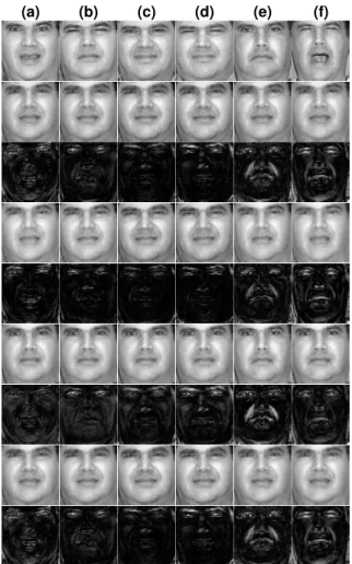
(a) (b) (c) (d) (e) (f)
Figure 6: Expression extraction for a single subject: Ex-pressive faces reside in row I. Identity classes produced by PCP, PSSV, PCPS, RPCAG are in rows II, IV, VI, VIII. The complementary expression components are depicted in rows III, V, VII, IX.
To begin with, evaluation was effected on the CMU Multi-PIE dataset. Aligned and cropped165×172images of frontal pose and normal lighting from 54 subjects were used. We batch-processed each subject forming a28380×6 observation matrix to extract expressions: Neutral, Smile, Surprise, Disgust, Scream and Squint. For each subject, side information was offered by a sextet of neutral face rep-etitions. Archetypal expressions recovered by PCP, PCPS, PSSV, RPCAG are laid out in Figure6(the restricted num-ber of expressions disallows FRPCAG). It is noteworthy that local appearance changes separated by PCPS are the most salient which paves the way for better classification. We avail ourselves of the multi-class RBF-kernel SVM and the SRC [30] to map expressions to emotions. 9-fold cross-validation results are reported in Table1. PCPS leads PCP by a fair margin with PSSV, RPCAG underperforming PCP.
Algorithm PCP PSSV PCPS RPCAG
Non-linear SVM 78.40 74.69 79.94 77.16
SRC 79.01 74.38 82.72 79.01
Table 1: Classification accuracy (%) on the Multi-PIE dataset for PCP, PSSV, PCPS and RPCAG by means of non-linear SVM and SRC learning.
Lastly, the CK+ dataset was incorporated to assess the joint face and expression recognition capabilities of various algorithms. Each test image is sparsely coded via a dic-tionary of both identities and universal expressions (Anger, Disgust, Fear, Happiness, Sadness and Surprise). The least resulting reconstruction residual thereupon determines its identity or expression. We refer readers to [12] for the exact problem set-up and implementation details. Table2collects the computed recognition rates. Although RPCAG and FR-PCAG are superior than PCP as expected, PCPS performs distinctly better than all others.
Algorithm PCP PSSV PCPS RPCAG FRPCAG
Identity 87.35 87.05 95.23 89.77 90.98
Expression 49.24 45.30 67.50 58.26 57.73
Table 2: Recognition rates (%) for joint identity & expres-sion recognition averaged over 10 trials on CK+
5. Conclusion
In this paper, we have, for the first time, assimilated side information of the same format as observation into the framework of Robust Principal Component Analysis based on trace norms. Existing extensions of subspace features have also been successfully amalgamated in a convex fash-ion. Extensive experiments have shown that our algorithms not only perform better where Robust PCA is effective but also remain potent when Robust PCA fails. Directions for future research include generalising to the tensor case and to components of multiple scales.
References
[1] S. An, W. Liu, and S. Venkatesh. Exploiting side information in locality preserving projection.CVPR, 2008.1
[2] A. Aravkin, S. Becker, V. Cevher, and P. Olsen. A variational approach to stable principal component pursuit. UAI, pages 32–41, 2014.1
[3] B. Bao, G. Liu, C. Xu, and S. Yan. Inductive robust principal component analysis. IEEE Transactions on Image Process-ing, 21(8):3794 – 3800, 2012.1
[4] S. Boyd, N. Parikh, E. Chu, B. Peleato, and J. Eckstein. Dis-tributed optimization and statistical learning via the alternat-ing direction method of multipliers.Foundations and Trends in Machine Learning, 3(1):1–122, 2011. 3
[5] R. Cabral, F. De la Torre, J. Costeira, and A. Bernardino. Unifying nuclear norm and bilinear factorization approaches for low-rank matrix decomposition.ICCV, 2013.1 [6] E. Cand`es. The restricted isometry property and its
impli-cations for compressed sensing.Comptes Rendus Mathema-tique, 346(9):589–592, 2008.1
[7] E. Cand`es, X. Li, Y. Ma, and J. Wright. Robust principal component analysis?Journal of the ACM, 58(3):11:1–11:37, 2011.1,3,4,7
[8] V. Chandrasekaran, S. Sanghavi, P. Parrilo, and A. Willsky. Rank-sparsity incoherence for matrix decomposition. SIAM Journal on Optimization, 21(2):572–596, 2011.1
[9] K. Chiang, C. Hsieh, and I. Dhillon. Matrix completion with noisy side information.NIPS, 2015.1
[10] K. Chiang, C. Hsieh, and I. Dhillon. Robust principal com-ponent analysis with side information. ICML, 2016. 1,2, 4
[11] I. Cox, J. Kilian, F. Leighton, and T. Shamoon. Secure spread spectrum watermarking for multimedia. IEEE Transactions on Image Processing, 6(12):1673–1687, 1997.1
[12] C. Georgakis, Y. Panagakis, and M. Pantic. Discriminant incoherent component analysis.IEEE Transactions on Image Processing, 25(5):2021–2034, 2016.8
[13] J. Jiao, T. Courtade, K. Venkat, and T. Weissman. Justifica-tion of logarithmic loss via the benefit of side informaJustifica-tion. IEEE Transactions on Information Theory, 61(10):5357– 5365, 2015.1
[14] W. Kang, D. Cao, and N. Liu. Deception with side informa-tion in biometric authenticainforma-tion systems.IEEE Transactions on Information Theory, 61(3):1344–1350, 2015.1
[15] G. Liu, Z. Lin, S. Yan, J. Sun, Y. Yu, and Y. Ma. Robust recovery of subspace structures by low-rank representation. TPAMI, 35(1):171–184, 2013.4
[16] R. Margolin, L. Zelnik-Manor, and A. Tal. How to evaluate foreground maps? CVPR, 2014.7
[17] J. Mota, N. Deligiannis, and M. Rodrigues. Compressed sensing with side information: Geometrical interpretation and performance bounds.GlobalSIP, 2014.1,2
[18] M. Nielsen and I. Chuang. Quantum computation and quan-tum information.Cambridge University Press, 2010.2 [19] T. Oh, Y. Tai, J. Bazin, H. Kim, and I. Kweon. Partial sum
minimization of singular values in robust PCA: Algorithm and applications.TPAMI, 38(4):744–758, 2016.4
[20] V. Patel, T. Wu, S. Biswas, P. Phillips, and R. Chellappa. Dictionary-based face recognition under variable lighting and pose. IEEE Transactions on Information Forensics and Security, 7(3):954–965, 2012.6
[21] C. Sagonas, Y. Panagakis, S. Zafeiriou, and M. Pan-tic. RAPS: Robust and efficient automatic construction of person-specific deformable models.CVPR, 2014.1,2,4 [22] A. Shabalin and A. Nobel. Reconstruction of a low-rank
matrix in the presence of gaussian noise. Journal of Multi-variate Analysis, 118:67–76, 2013.4
[23] N. Shahid, V. Kalofolias, X. Bresson, M. Bronstein, and P. Vandergheynst. Robust principal component analysis on graphs.ICCV, 2015.2
[24] N. Shahid, N. Perraudin, V. Kalofolias, G. Puy, and P. Van-dergheynst. Fast robust PCA on graphs. IEEE Journal of Selected Topics in Signal Processing, 10(4):740–756, 2016. 2
[25] F. Shang, Y. Liu, J. Cheng, and H. Cheng. Robust principal component analysis with missing data. CIKM, pages 1149– 1158, 2014.1
[26] V. Stankovi´c, L. Stankovi´c, and S. Cheng. Compressive im-age sampling with side information.ICIP, 2009.1 [27] H. Sun, J. Wang, and T. Deng. On the global and linear
convergence of direct extension of ADMM for 3-block sep-arable convex minimization models. Journal of Inequalities and Applications, (227):227, 2016.3
[28] S. Taheri, V. Patel, and R. Chellappa. Component-based recognition of facesand facial expressions. IEEE Transac-tions on Affective Computing, 4:360–371, 2013. 8
[29] G. Warnell, S. Bhattacharya, R. Chellappa, and T. Bas¸ar. Adaptive-rate compressive sensing using side information. IEEE Transactions on Image Processing, 24(11):3846–3857, 2015.1
[30] J. Wright, A. Yang, A. Ganesh, S. Sastry, and Y. Ma. Ro-bust face recognition via sparse representation. TPAMI, 31(2):210–227, 2009.8
[31] L. Wu, S. Hoi, R. Jin, J. Zhu, and N. Yu. Distance metric learning from uncertain side information with application to automated photo tagging.ACMMM, 2009.1
[32] A. Wyner and J. Ziv. The rate-distortion function for source coding with side information at the decoder.IEEE Transac-tions on Information Theory, 22(1):1–10, 1976. 1
[33] H. Xu, C. Caramanis, and S. Sanghavi. Robust pca via
outlier pursuit. IEEE Transactions on Information Theory, 58(5):3047–3064, 2012.1
[34] M. Xu, J. R, and Z. Zhou. Speedup matrix completion with side information: Application to multi-label learning.NIPS, 2013.1
[35] L. Zhang, L. Wang, and W. Lin. Conjunctive patches sub-space learning with side information for collaborative im-age retrieval. IEEE Transactions on Image Processing, 21(8):3707–3720, 2012.1
[36] Z. Zhou, X. Li, J. Wright, E. Cand`es, and Y. Ma. Stable principal component pursuit.ISIT, 2010.1