A Novel Power Amplifier Behavior Modeling Based on RBF Neural Network with Chaos Particle Swarm Optimization Algorithm

A Novel Power Amplifier Behavior Modeling

Based on RBF Neural Network with Chaos

Particle Swarm Optimization Algorithm

Mingming Gao

School of Electrics and Information Engineering, Liaoning Technical University, Huludao, China E-mail:[email protected]

Jingchang Nan

School of Electrics and Information Engineering, Liaoning Technical University, Huludao, China E-mail:[email protected]

Surina Wang

University of British Columbia, Vancouver, Canada E-mail:[email protected]

Abstract—In order to design and optimize high-linearity power amplifier (PA), which with nonlinear and memory effect, it is very important to build power amplifier behavior modeling accurately. This paper proposes a power amplifier behavior modeling based on RBF neural network with improved chaos particle swarm optimization algorithm. To make the particles evenly distribute in the problem search space, a novel Chaos Particle Swarm Optimization (CPSO) is proposed based on the analysis of the ergodicity of chaos and inertia weight of Particle Swarm Optimization (PSO). Based on circle model, the new model is introduced to avoid PSO from getting into local optimum. This paper uses free scale semiconductor chip MRF6S21140 to carry on amplifier circuit design in the ADS and the MATLAB fitting simulation of the extracted data, by improved CPSO-RBF algorithm. Its accuracy is assessed by comparing RBF modeling with voltage RMS error (RMSE), epochs, and fitting time. The result shows that improved CPSO-RBF has better fitting function.

Index Terms—Power Amplifier; CPSO; Neural Network; Behavioral Model

I. INTRODUCTION

With the development of modern communication technology, many communication systems use high efficient spectrum techniques. These techniques have a high peak to average power ratio, in order to increase the transfer rate and channel capacity, that is, efficient digital modulation formats (such as M-QAM and OFDM) and new multiple access methods (such as OFDMA, MC-CDMA, and WCDMA). The power amplifier device will produce nonlinearity and memory effects because of these techniques. In order to linearize the nonlinear power amplifier system, an accurate power amplifier behavior model is to be obtained. Thus, the behavior modeling

techniques, which can deal with both nonlinear and memory effect, have become one of the hot topics in interdisciplinary research, including: microwave applications, wireless communications, radar, semiconductor physics, nonlinear control, and instrumentation.

In behavioral modeling, for example, one of the challenges of the modeling of nonlinear behavior of RF microwave modules is to precisely describe both strong nonlinearity and memory effects, which have more time on the dynamic characteristics of a constant or combination [1-3]. Power amplifier is a critical nonlinear module in various radio frequency communication systems. In an efficient modulation system, the fact demonstrates that power amplifier is not only characteristic of nonlinearity but also of strong memory effects. Therefore, how to precisely model memory effect in dynamic nonlinear amplifier is an important problem. There are lots of reports on RF power amplifier modeling both at home and abroad, which include memoryless model, Volterra-Series model and its Simplified model, different types of neural network model, and so on[4-6]. Compare to Volterra series model, neural network model has good approximation capabilities. It can better describe the behavior of weak and strong nonlinear amplifier models, and the result can be generalized. One of the advantages of RBF neural network model is that it can be applied to any nonlinear function, and it is also suitable for power amplifier model building. In RBF neural network model, we need to determine the structure parameters, which are the center bits of basis function, the variance, and network weights[7,8].These parameters will determine the performance of the neural network. Particle Swarm Optimization (PSO) algorithm uses the same speed model as the position search, which is fast, accurate, and concise, and has low computational complexity and easy implementation. Particle Swarm Optimization (PSO) algorithm will search for global

Project number: No.61372058; LR2013012;MTKJ2011-339 Contact author: Mingming Gao

Output ( )

x l

( 1)

x l −

( )

x l−L

ϕ

2

ϕ

#

∑

∑

1

ϕ

=

#

Input

Hidden

,2

M

ω

1,1

ω

1,2

ω ω2,1

0.1 b1

ω =

0.2 b2

ω =

,1

M

ω

2,2

ω

1

ϕ

Figure1. RBF Neural Network model block diagram

optimal solution through groups of particles in cooperation and competition. In order to improve the performance of neural network training, researchers at home and abroad used Particle Swarm Optimization (PSO) algorithm to train neural network weights and topology. However, the basic PSO algorithm in slow fitting is close to the optimal solution, which is easy to appear and even to a standstill, and makes the network training difficult to achieve the desired effect. Hence, many scholars proposed a modified PSO algorithm. Currently several improved algorithms have been made, such as adaptive PSO algorithm, hybrid PSO algorithm, collaborative PSO algorithm, discrete PSO algorithm, and immune PSO algorithm. Chaos in a nonlinear phenomenon is widespread in nature: it appears to be chaotic, but has exquisite internal structure; it has randomness, ergodicity, and regularity characteristics, and it is extremely sensitive to initial conditions; it can change according to its own laws within a certain range and will not repeat to loop through all state. These properties can be optimized using chaotic motion search.

This paper is organized as follows: in Section II, the paper proposes a novel chaotic Particle Swarm Optimization algorithm, by combining with the RFB neural network to build power amplifier behavioral modeling. In Section III, the paper proposes a power amplifier behavior modeling based on RBF neural network with improved chaos particle swarm optimization algorithm (CPSO-RBF). In Section IV, the paper shows the simulation results of CPSO-RBF power amplifier modeling has higher precision. Finally, in Section V, a conclusion is presented.

II POWER AMPLIFIER NEURAL NETWORK MODEL OF RBF AND THE LEARNING ALGORITHM

A. The Expression of RBF Neural Network Model of Power Amplifier

This model is the selection of General RBF Neural networks. RBF Neural network is consisted of input layer, hidden layer, and output layer. In this model, input amplifiers of complex signals are converted to amplitude and phase of a polar form, and then are trained on the real-valued amplitude and phase. According to the amplifier's nonlinear characteristics and memory effects of power amplifier, the amplifier output expression is:

( ) ( ( ) , ( 1) , , ( ) )

exp{ [ ( ) [ ( ) , ( 1) , , ( ) ]]}

y l g x l x l x l L

j l f x l x l x l L

= − − ×

Φ + − −

"

" . (1)

|x(l)| and Φ(l) are the input signal amplitude and phase

respectively, L is the memory effect in a memory depth, which is the number of models in the previous sample. Nonlinear power amplifier can be expressed by AM/AM and AM/PM characteristic curves. There are two corresponding output nodes for AM/AM and AM/PM nonlinear distortion functions, g() and f(), that can

describe the dynamic characteristics of power amplifier’s AM/AM and AM/PM.

RBF Neural network has L+1 entries input notes, which is X=[|x(l)|,|x(l-1)|,…,|x(l-L)|]T_{. It supposes based}

training samples for n, and it’s hidden layers have M

(M<N) neurons. Any one of the neurons indicated by i,

φ(X,Ci) is the primary function which for the ith

motivation of hidden units in output. Hidden output layer weights can be provided by ωji. Output unit also set a threshold φ, in order to suppress floor G0 of a neuron's

output as 1, the output unit is attached to the right value for ω0i. The model structure is shown in Figure 1:

Function φ(X,Ci) generally selectes basis on Green's

function, using the definition of Green's functions

2

2

( ) exp( )

2 i i

i

x c G x c

σ

−

− = − to indicate the hidden layer of

non-linear function {φi(x)=G(||X-ci||), i=1,2,…,M}. M is

the number of hidden layer of units, X is the input vector, {ci|i=1,2,…,M} is the central point of G(), and σi is the

field width of the ith _{hidden node. The j}th _{(j=1,2) output}

node of the output is:

1

( ) L _ji ( _i ) _j

i j

y x _ω G x c b

=

=

∑

Among them, ωji is the weight that connects between the hidden layer of ith _{nerve cell and output layer of the j}th

neuron, and bj is the ground term. Smoothness of the

approximation is depended on 2

i σ .

The number of real parameters to M(L+3)+2 of RBF Neural network can show the nonlinear dynamic behavior of the power amplifier.

B. Improved Chaos Particle Swarm Optimization Algorithm

Set in the group, the ith _{Particles is x}

i (xi1, xi2, …, xid)

with experienced location pi (pi1, pi2, …, pid), and for

individuals the best location is pbest. Currently, all particles that make up the groups have experienced the best location pgbest, and grain ith_{’s speed can provide by}

vi(vi1, vi2, …, vid). On each iteration, the grain ith in d

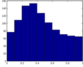
0 0.2 0.4 0.6 0.8 1 0

50 100 150 200 250

Figure 2. Logistic distribution by iterated 1000 times

0 0.2 0.4 0.6 0.8 1

0 20 40 60 80 100 120 140 160

Figure 3. Circle distribution by iterated 1000 times

0 50 100 150 200

0 20 40 60 80 100 120

Figure 4. The new map distribution by iterated 1000 times

1

1 ()( ) 2 ()( )

k k k k k

id id id id gbest id

v +₌ωv ₊cRand p x_{− +}c Rand p ₋x _{. (3)}

1

k k k

id id id

x + ₌x ₊v _{. (4)}

In formula (3), ω is the inertia weights, which keeps the particles movement inertia, and ωgives it the ability to explore new areas; c1 and c2 are acceleration constants, their values are usually between 1.5-2, and the algorithm takes the value of 2. They allow each particle’s accelerated motion to pbest and pgbest locations. Rand () represents random numbers, which ranges form (0, 1).

Chaos in a nonlinear phenomenon is widespread in nature, and the more commonly used model is the chaos model of logistic model, whose expression is:

1 (1 ) 1, 2,

n n n

X + =μX −X n= ". (5)

The following figure is a performance chart image of logistic, when μ=4. Logistic map is iterated 1000 times within the range of (0, 1) map. Figure 2 shows 0, 0.1, and 0.9, 1 with high probability interval value, where the highest probability point could reach 212 times. However, between 0.1 to 0.9, the average probability point is 76 times. When the optimal value falls between 0.1, and 0.9, we need a number of iterations to get the optimal solution, and this greatly reduces the efficiency of algorithms.[9]

However, logistic model produces uneven distribution of chaos, and round mapping model Traverse with good uniformity. The equation is as follows:

[

]

1 ₂ sin 2 mod1

n n n

a

X X b _πX

π +

⎡ ⎤

= + −_{⎢ ⎥}

⎣ ⎦ . (6)

Following figure 3 is the allocation plan of Circle map by iterated 1000 times. Among them, a=0.5 and b=0.2. The probability of 0-1 point is as shown in figure 3. It can be perceived that the maximum number is 151 times, minimum is 63 times, and the average is about 100 times, which is higher than logistic mapping but less than uniform probability distribution.

In order to further improve the adequacy and traversal of chaotic search, this paper presents a new map, which can be written as the following formula:

[

]

1 (1* ₄ sin 4 ) mod1

n n n

a

X X b πX

π +

⎡ ⎤

= + −_{⎢ ⎥}

⎣ ⎦ . (7)

Figure 4 is the new model, mapping iterative 1000 times and 0-1 range of distribution. You can see from the figure, the maximum value is 115 times and minimum is 94 times. The new model is better than the basic Circle

map and the logistic map on mapping efficiency, and it distributes more evenly.

Chaos Particle Swarm Optimization is mainly reflected in the application of the paper: By using the new model, it can have a uniform distribution of chaos, initialized to population, and inertia weight. ωis an important parameter in Particle Swarm Optimization algorithm, with evolutionary adaptive adjustment of the value of ω, formula sets as follows:

[

]

1 1* ₄ sin 4 mod[1] 0.2

n n n

a

X X b πX

π +

⎡ ⎤

= + −_{⎢ ⎥} +

⎣ ⎦ .(8)

In formula (8), K is the number of iterations. The detailed algorithm is as follows:

Step 1. Initial population. Set the population size to be N, the particle dimension to be D, and assign initial values with small differences to the chaotic equation (7) of i, then we can get a chaotic variable xi; and by changing the ith variable on the interval of Xmin, Xmax map to the location variable values, we can build location variable.

Vout Vin V_DC SRC2 Vdc=28 V VAR VAR2 tstep= 1/(4*SymbolRate) RF_Freq= 2140 MHz SymbolRate=3.84 MHz RFpower_dBm=30 Eqn Var Envelope Env1 Step=tstep Stop=1000/(SymbolRate) Order[1]=5 Freq[1]=RF_Freq ENVELOPE R R2 R=50_Ohm V_DC SRC3 Vdc=4 V MSUB MSub1 Rough=0 mil TanD=0.0005 T=0.035 mm Hu=3.9e+034 mil Cond=5.88e7 Mur=1 Er=3.5 H=0.76 mm MSub FSL_TECH_INCLUDE FTI FSL_TECH_INCLUDE MRF-thermal-effect X6 CDM A 2 000 MRF5P21180 X7 Port P4 Num=4 Port P2 Num=2 MLIN TL49 MLIN TL48 C C16 R R6 R R3 R R4 FSL_MRF_MET_PP_MODEL MRF1 R R1 R R5 MLIN TL51 MLIN TL47 C C38 MLIN TL46 C

C20CC21 CC22 CC23

C C19 C C18 C C30 MLIN TL50 MLIN TL45 C C28 C C26 C C29 C C27 C C25 C C24 MLIN TL44 MLIN TL52 Port P3 Num=3 C C32 C C31 C C33 C C34 C

C14 CC15 CC17

MLIN

TL43

Port

P1 Num=1 MLINTL30

MLIN

TL31

MLIN

TL32 CC37 MLINTL33 MLINTL34

MLIN TL40 C C36 MLIN TL39 MLIN TL38 MLIN TL42 MLIN TL37 MLIN TL36 MLIN TL35

Figure5. Power amplifier circuit schematic

5 10 15

0 20 20 40 60 80 0 100 time, usec mag( V fun d_in) m a g( V fund _out ) mag(Vfund_in) mag(Vfund_out)

Figure 6. The input and output voltage of power amplifier

0 10 20 30 40 50 60 70 80 90 100 -10 0 10 20 30 40 50 60 70 80 90 100

the number of sample

out put v ol tage am pl it ude( v )

actual messured value RBFmodel output value error

Figure 7. Fitting result of voltage range based on RBF model

fitness value to be the corresponding global extreme value, gbest.

Step 4. Use formula (8) to calculate the inertia weight valueω, in formula (3).

Step 5. Update the speed and position of the particle according to formulas (3) and (4).

Step 6. The fitness value of each particle will be compared with the existing pbest value. If the new value is better, then replace the existing pbest value, otherwise, retain the original values; select the individual with the optimal fitness in pbest to be gbest.

Step 7. Determine whether the fitting criteria is met, if yes, terminate the optimization process and output the result; otherwise return to step 2.

III THE ALGORITHM OF RBFNEURAL NETWORK WITH

IMPROVED CHAOS PARTICLE SWARM OPTIMIZATION

The performance of RBF network is determined by the parameters of the network, which is the center and variance of the basis function as well as network weights [10]. If the chaotic particle swarm algorithm is used for neural network training, then it is not easy for particles to get into the local optimum [11-12]. This algorithm can also expand the search space, search the global optimal solution, and speed up the fitting rate of the neural network training algorithm. Specific optimization (improved CPSO-RBF) procedures are as follows:

a) Preprocess the sample, and normalize the sample data value to the range between 0 and 1.

b) Initialize the network structure; then the parameters of wi, ci, σi will constitute particles and give them random

values to initialize the size, location, and speed of the particle swarm.

c) After getting the input/output response value of RBF neural network, calculate the fitness value of particle swarm according to fitness value formula of fitness to determine the optimal value of individual and population.

N denotes the number of the training samples, D denotes the number of output neurons, yij and tijdenote the output

value, and the expected output value of the jth _component

of the ith _{sample respectively.}

d) Update the position and speed of population particles according to the formulae (3) and (4), and then produce new particle swarm.

e) Judge whether the result meets the optimization goal or maximum number of training, if it meets the termination conditions, then terminate the algorithm; otherwise returns to c.

IV THE SIMULATION RESULTS OF POWER AMPLIFIER

BEHAVIOR MODELING

It uses the MRF6S21140 semiconductor transistor of free scale for power amplifier circuit design. Based on the design of the circuit, CDMA2000 source is used for enveloping simulation. The amplifier circuit schematic is shown in figure 5. Figure 6 shows that due to the inherent nonlinear of power amplifier, there is a certain degree of distortion of output signal corresponding to the original input signal of power amplifier. In order to modeling

power amplifier, we must take the waveforms of input/output voltage amplitude. In the process of the neural network training, it needs to use the amplifier's input voltage amplitude as neural network input and the amplifier's output amplitude as expected output of the neural network.

Choose the input/output of the power amplifier with the greatest amplitude to build the new model. The experiment uses 90 data points to facilitate the simulation of neural network, and we select memory depth M=3.

It extracts 200 groups of input and output voltage amplitude values from the power amplifier circuit design, compares the fitting degree of input/output voltage amplitude of RBF, and improves CPSO_RBF power amplifier models according to the selected voltage from amplifier circuit. Analyze the simulation results and fit the simulation results. The results include: voltage amplitude output value and output error. It shows the curves of fitting result of voltage range based on RBF model in figure 7, the curves of fitting result of voltage

0 10 20 30 40 50 60 70 80 90 100 0

20 40 60 80 100

the number of sample

out

p

ut

v

ol

tage am

pl

it

ud

e(

v

)

actual messured value CPSO-RBF model output value error

Figure 8. Fitting result of voltage range based on CPSO-RBF model

0 20 40 60 80 100 120 140 160 180 200 0

0.005 0.01 0.015 0.02 0.025 0.03

evolution algebra

fi

tn

e

s

s

Fitness curve MSE[PSOmethod] (parameter c1=1.5,c2=1.7,termination of algebra=200,populationpop=20)

Best c=8.247 g=12.9901 CVmse=0.0042667

the best fitness the average fitness

Figure 9. Fitness curve of improved CPSO-RBF model

Figure 10. Epoch curve of improved CPSO-RBF model

TABLE I.

THESIMULATIONRESULTSOFRBFANDCPSO-RBF MODELINGBASEONVOLTAGEAMPLITUDE

Items RBF CPSO-RBF

RMSE 0.0042 0.0027

Epochs 12 20

Fitting time(s)： 2.00 3.00

-6 -4 -2 0 2 4 6

x 106 -40

-35 -30 -25 -20 -15 -10 -5 0

Frequency(Hz)

PSD

(H

z

/d

B

)

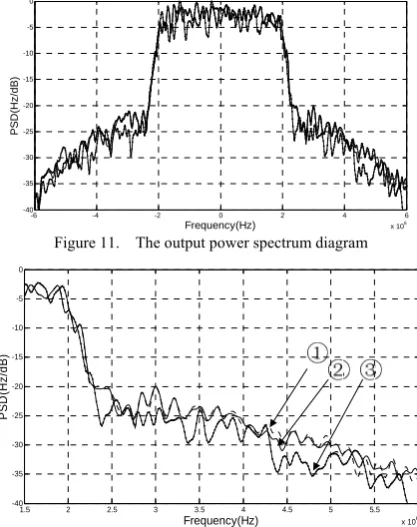
Figure 11. The output power spectrum diagram

1.5 2 2.5 3 3.5 4 4.5 5 5.5 6 x 106 -40

-35 -30 -25 -20 -15 -10 -5 0

Frequency(Hz)

PS

D

(H

z

/d

B

)

Figure 12. The local enlarged spectrum diagram

By contrasting figure 7 and figure 8, we can see that improved CPSO-RBF modeling has better fitting effect than RBP modeling. Improved CPSO-RBF modeling can simulate the power amplifier more accurately. It optimizes RBF neural network weights for global by improved CPSO algorithm, and overcomes the problems in training accuracy and speed of RBF. By comparing the actual output voltage with the simulated output voltage map, the simulated data of improved CPSO-RBF modeling is close to the measurement and is quite consistent. The effect of memory is also being considered

in the simulation process, and thus, this modeling can simulate the nonlinear and memory effects of the power amplifiers. Improved CPSO-RBF modeling, which increases training frequency, has longer time-consumption. Voltage RMS error (RMSE) is compared between improved CPSO-RBF modeling output and RBF modeling output of amplifier to validate the model accuracy. Also, we compare epochs and fitting time to validate the modeling training speed. Obviously, this error can be controlled in a small numerical range, and fitting time can be maintained in a short time.

The output power spectrum diagram of the amplifier model of improved CPSO-RBF modeling and RBF modeling is shown in figure 5 (a), and figure 5 (b) is the local enlarged spectrum diagram of figure 5 (a). In figure 5 (b), curve ① is for actual output power spectrum of amplifier, curve ② is output power spectrum for RBF model calculation, and curve i③ s the output power spectrum for improved CPSO-RBF model calculation. It can be seen that improved CPSO-RBF model’s output power spectrum of amplifier is better and closer to the actual power spectra model performance by the simulation results.

V CONCLUSIONS

amplifiers precisely. Hence, this modeling could be used for the linearization of power amplifier system, and it is crucial for practical designing purpose.

ACKNOWLEDGMENT

This work is supported by National Natural Science Foundation of China (No.61372058), Talent fund projects in Liaoning province (LR2013012), China coal industry association of science and technology research plan projects(MTKJ2011-339)and the earlier stage funding for the natural science foundation of the Liaoning Technical University in 2011.

REFERENCES

[1] J. C. Pedro et al, “A Comparative Overview of Microwave and Wireless Power-Amplifier Behavioral Modeling Approaches,” IEEE Transactions on Microwave Theory and Techniques, Vol.53, No.4, April 2005.

[2] Zhang Jing, He Song-bai and Gan Lu. Design of a

memory polynomial predistorter for wideband envelope tracking amplifiers [J]. Journal of Systems Engineering and Electronics, 2011, 22(2): 193-199.

[3] Hui Feng, Zeqi Yu. “The Correction Method for Power

Noise in Digital Class D Power Amplifiers”, Journal of Software, Vol. 8, No. 2, pp:488-494,2013.

[4] Farsaei A R, Safian R. An effective method for generating initial condition in harmonic balance analysis using method of nonlinear currents[C]. Microwave Conference, Dec.2009:1501-1504.

[5] O. Hammi, F. M. Ghannouchi, and B. Vassilakis, A

compact envelope memory polynomial for RF transmitters modeling with application to baseband and RF-digital predistortion [J], IEEE Transactions on Microw.Wireless Compon.Lett., 2008, 18(5):359–361.

[6] NAN Jing-chang, GAO Ming-ming; LIU Yuan-an,

“Analysis and Comparison of Behavioral Models for Nonlinear RF Power Amplifier, ” Journal of Microwaves, 2008.S1

[7] LI Jiu-chao; NAN Jing-chang, LIU Yu-an, “Study of

Memory Effects on Power Amplifier for Communication System,” Computer Simulation, 2010.7.

[8] WANG Yan, SUN Xiang feng, “LI Ming, Training

Method for Support Vector Machine Based on Chaos Particle Swarm Optimization,” Computer Engineering, Vol. 36, No. 23, 189-191, December 2010.

[9] Zhihui Zhan, Jun Zhang, Yun Li, et al. Adaptive Particle Swarm Optimization [J]. Transctions on Systems, Man and Cybernetics, 39(6), 2009:1362-1381.

[10] TIAN Yubo, LI Zhengqiang, ZHU Renjie, “Selective

neural network ensemble methods based on chaos PSO,” Computer Applications, Vol. 28, No. 11, 2844-2846, Nov. 2008.

[11] Liangyou Shu, Lingxiao Yang.” A Modified PSO to

Optimize Manufacturers Production and Delivery” ,Journal of Software, Vol. 7, No.10, pp:2325-2332,2012.

[12] Xuewen Xia, Jingnan Liu, Yuanxiang Li.” Particle Swarm Optimization Algorithm with Reverse-Learning and Local-Learning Behavior”, Journal of Software, Vol. 9, No.2, pp:350-357,2014.

Mingming Gao was born in 1980,

China. She is a Ph.D. candidate in Liaoning Technical University. Also she is a lecturer in School of Electronic and Information Engineering, Liaoning Technical University. She obtained her Master Degree from Liaoning Technical University in 2008. She is interested in wireless communications, coalmine disaster forecast and communication, etc.

Jingchang Nan was born in 1971, China,

a professor from Liaoning technical university. He received the B.Eng degree in industrial electric antomation from Liaoning technical university, Fuxin City, Liaoning Province, China, in 1993, and received the M.S (signal and information processing) and Ph.D degrees (electromagnetic field and microwave technology) from Liaoning technical university and Beijing university of post and telecommunication, in 2003 and 2007, respectively.

He began teaching in Liaoning technical university from 1993, and was engaged in teaching and research of communication engineering in 1994. So far, he authored and co-authored over 40 papers in international conferences and journals, including ICCP, MAPE, ICMMT, J. of electromagn. Wave and appl., J. of electronic and information, High technique letters, and so on. He has presided over some important subjects and researches, including the national natural foundation of China, Dr start fund project of science and research for Liaoning province. He is interested in RF circuit and system, communication system and

simulation, adaptive signal and information processing.

Surina Wang, was born in 1983,