Optimal design of high speed mechanical systems

(1)

Optimal Design of High Speed Mechanical Systems

by

J.W. David, C.Y. Cheng, T.D. Choi, C.T. Kelley, and J. Gablonsky

Departments of Mechanical and Aerospace Engineering and Mathematics

Center for Research in Scientific Computation

North Carolina State University

ABSTRACT

The trend towards higher performance mechanical systems has naturally led to the need to design such systems in an optimal fashion. Lighter components and higher operating speeds both demand a level of design a step above that provided conventionally. This paper describes a research effort aimed at developing the methodology for such system design. The methodology is based on accurate computer modeling, experimental validation, and robust optimal design strategies along with a parallel computing environment to produce optimal mechanical systems. As an example, a valve train mechanism used in high speed racing engines is analyzed and optimized. Experimental validation of the optimized designs is also presented.

INTRODUCTION

As the pace of modern society increases, so does the need for high speed machinery. Increased manufacturing capacity, increased transportation speeds and the ever present ‘more, better, faster’ mentality of modern life demands ever increasing sophistication of mechanical equipment. Even with the advent of modern computer-aided design tools, the dynamic design of machines is today very similar to that of thirty years ago. Machines are designed based on the ingenuity of the design engineer, computer and experimental tools are used to refine the design, and the machine is built. Optimality of the design is seldom considered, though it is approached through continued refinement. The work presented in this paper attempts to provide a design methodology by which mechanical systems may be optimized early in the design stage, before production begins, to produce higher performance. To demonstrate the

methodology, a high speed automotive valve train system is optimized for increased engine performance.

MODELING ISSUES

Computer models have emerged in the last 30 years as the premier tool for analyzing mechanical systems. The advent of the finite element method has given machine designers a powerful tool for mechanical system analysis. However, since optimal design often requires millions of simulations, the modeling process must be approached carefully. A large scale computer model, with thousands of degrees of freedom, would require so much computational effort on even the fastest computer so as to render optimal design impractical. Thus, optimal design transfers some requirement for ingenuity from the designer to the analyst. The computer model for the system at hand must include sufficient detail to include important system characteristics while limiting the number of degrees of freedom.

(2)

other concerns are most important. Initial studies of this mechanism yielded models with many degrees of freedom [1]. In addition, in order to obtain steady-state responses from a numerical integration of the equations of motion, the simulation required several cam cycles. For the computers available at that time, over two minutes of

cpu time were required to simulate the mechanism at one camshaft speed. In that the mechanism was to be optimized over several camshaft speeds (over 20), this was prohibitive.

Thus, the computer model developed for this problem needed to be computationally efficient as well as accurate. Figure 2 shows a schematic of the model developed for this study [2]. It is uses a frequency response function approach for the valve spring dynamics, thus achieving steady state response in on cam cycle simulation. The valve spring frequency response function also reduced the degrees of freedom to 3, on for the lifter, one for the rocker arm and one for the valve. The pushrod mass is lumped, half to the lifter and half to the rocker arm. The stiffness and damping coefficients represent the physical characteristics of the components. As this mechanism often forms gaps between connecting components, it was deemed important to include such effects in the model. To do this, the kinematic relationships between the contacting elements are constantly monitored and, when a connecting joint would be required to

transmit a tensile force, the interconnecting spring and damping coefficient are set to zero. Transitions from contact to non-contacting are handled with a variable step Runge-Kutta numerical integration algorithm. For this model, the cpu time was reduced to 6 seconds per engine speed. The issue of accuracy must still be proven.

PARAMETER IDENTIFICATION

The computer model of Figure 2 has many input parameters. Some, such as physical dimensions and masses, are easily measured. The stiffness coefficients are somewhat more difficult to measure. The damping coefficients are extremely difficult to

measure directly

and thus, a system identification approach is taken in this study to obtain the stiffness and damping coefficients. This includes k1 through k4 (k5

represents an additional spring and thus is easily determined) c1 through c4 and the friction

coefficients for the rocker arm pivot, valve stem, and valve spring. Thus, a total of 11 parameters must be determined for this model.

As this system is highly nonlinear (many contact and separation events), traditional modal analysis techniques are not helpful. The approach taken here is to form an objective function which measures the difference(s) in response between the model and experiment and then adjusts the system parameters to minimize this function. Several issues become apparent here, the system response variable to measure, the form of the objective function, and the optimization algorithm.

Figure 1 A Typical Pushrod Valve Train [1]

(3)

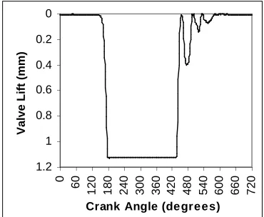
With the range of sensors available (strain gages, accelerometers, various displacement transducers), many measurements are possible. In that the goal of the mechanism is to open and close the valve in a controlled fashion, and that the dynamic dysfunction is characterized by uncontrolled valve motion, it would seem logical to measure the valve motion. Figure 3 shows the typical output from a short-range eddy current probe. The engine speed for this measurement is approximately 8,500 rpm. It has a reduced measuring range from a typical long-range probe, but provides improved resolution in the valve bounce area. Notice that the valve begins to open, and then exceeds the measurement range of the sensor at slightly over 1mm. Thus, the sensor produces a constant output even though the valve continues to move. As the valve closes, it reenters the measurement range of the sensor. Notice the valve opens, closes, and then reopens or ‘bounces’. This bounce is caused by residual vibration in the mechanism as well as high impact velocities between the valve and seat. This valve bounce is detrimental to the system operation and thus characterizes the level of dynamic dysfunction in the mechanism. In this case, the valve actually bounces 3 times after first closing. Data are taken with the short-range sensor at multiple engine speeds (typically 20 to 30) and each engine speed has 720 valve lift measurements.

0

0.2

0.4

0.6

0.8

1

1.2

0

60

120 180 240 300 360 420 480 540 600 660 720 Crank Angle (degrees)

Valve Lift (mm)

Figure 3 Typical Short-Range Sensor Ouput

Figure 4 shows a plot of valve bounce as a function of engine sped. This provides a concise representation of the dynamic performance of the mechanism. Notice that, in this case, the mechanism

is relatively stable up to about 7,800 rpm and then enters a region of varying valve bounce up to 9,100 rpm, where the mechanism becomes unstable as characterized by an ever increasing valve bounce amplitude.

OBJECTIVE FUNCTION

Because the system is transient and highly nonlinear, the parameter identification is cast as a least squares error between the predicted response of the model and the experimental data. This error is summed over the

0 0.1 0.2 0.3 0.4 0.5 0.6 0.7 0.8

7000 7500 8000 8500 9000

Engine Speed (rpm)

Maximum Valve Bounce (mm)

Figure 4 Valve Bounce Variations with Engine Speed

number of data points and number of test engine speeds:

f w y j_j _i y_i j j

npoints

i nspeed

= −

=

∑

( ( ) *( ))2 1

1

(1)

where yj is any predicted system response and yj* is

the corresponding measured response. The weighting function wj is included to exclude the data

(4)

between the measured and predicted responses. In an ideal situation with no modeling misconceptions or numerical errors, the cost function would be zero.

THE OPTIMIZATION PROBLEM

Figure 5 shows a plot of the cost function (equation 1) vs two of the system parameters. Notice that the topology has a dominant trend, but with many local minima. In that the global minimum of equation 1 is desired, an algorithm must be used capable of avoiding entrapment in the local minimum. To this end, an implicit filtering algorithm, developed by Gilmore and Kelley[4] was employed.

Figure 5 Cost Function Variation with Two System Parameters [3]

Implicit filtering is an implementation of the gradient-projection [5] algorithm which uses finite difference gradients with a sequence of difference steps to ``jump over'' local minima and avoid entrapment by high-frequency low-amplitude (and possible discontinuous) perturbations (which we will refer to as noise) of smooth objective functions. Such noise can arise, for example, from tabular interpolation of measured data or truncation errors in computations done inside the objective function. In this paper a parallel implementation of the algorithm is presented for the first time. The algorithm will be presented in some detail as to clearly present the natural parallelism. The problem to be solved is

min ( )

x∈ΩΩ

f

x

(2)

where x is the unknown and constraints on x are given by

Ω

Ω =

{

x l

i

≤ ≤

x

i

u

i

}

(3).

The meaning of equation 3 is that the ith component of x is bounded from above and below by the ith component of the vectors l and u. One can project x onto the feasible set Ω using

P ( )

i

i i i

i i i i

x

l

x

l

u

x

u

x

l

x

u

=

≤

≥

<









if

(4)

The gradient projection method transforms a current approximation

x

_c to the optimal point to a new iteration

x

₊ by

x

₊

=

P x

(

c

−

α ∇

∇

f(

x

c

)

(5)

where

α

is a step-length parameter. The new iterate is accepted if equation 6 holds, for some sufficiently small sigma (typically .0001).

f

(

x

_c

)

−

f

(

x

₊

)

≥

σ

x

c

−

x

+

α

2

(6)

If the iteration is rejected, the step-length parameter alpha is reduced.

Implicit filtering, by using a difference approximation to the gradients, offers a simple opportunity for parallelism by evaluating the functions in the difference simultaneously. The code presented here, IFFCO (Implicit Filtering For Constrained Optimization), [4,6], uses finite differences to approximate the partial derivatives of f. It uses central differences when it is able to and forward or backward when it must. For example, the centered difference approximation is given by

(

∇

h

( ))

=

(

+

)

−

(

−

)

h

f

i

f

i i

x

e

x

e

2

(7)

(5)

x

₊

−

x

_c

≤

τ

h

(8)

holds or too many iterations have been taken. At that point h is reduced and the projected gradient iteration is restarted using the best solution found so far as the initial iterate. The resolution (or sensitivity to high frequency terms) in the algorithm is therefore increased as the iteration progresses. Once convergence is attained at the minimum difference increment specified by the user, the options are either to accept the result or restart. The convergence theorems from [4] states that after finitely many restarts the entire sweep of the algorithm will leave the best point unchanged and that if the objective function is in a certain class of perturbations of smooth functions, the final result will be as close to a global minimum as the noise will allow. For the problem presented in this paper, one or two restarts were useful.

The situation where either a forward or backward difference must be used arises when one of the points that must be evaluated to compute the central difference is outside the constraint space. In the central difference case f must be evaluated twice. In the forward and backward differences f must be evaluated only once because x is the current point and f(x) is already known. This must be done for every component of the gradient. Thus, f must be evaluated at least n times and at most 2n times. Now, since the components of the gradient are completely independent of each other, they can be evaluated separately and simultaneously on different processors or computers.

PARALLEL COMPUTING

For parallel computing, a CRAY T3-D computer was used. IFFCO scales both the constraints and the function to make Ω a unit cube and the size of f at the initial iterate roughly 1. Having made this scaling, a sequence of difference increments was used, beginning with h = 0.2 and halving until h = .03125. The constraints were changed before some restarts. This is a different type of restart than that considered in [4] and [6]. One restart of this type was sufficient. The parameter τ in the termination criterion (8) is critical to effective use of the code. If

τ is too small, the iterations will not terminate successfully; if τ is too large the iteration can stagnate in a local minimum. This parameter is best selected by trial and error and τ = 0.1.

For a given difference increment, there are two kinds of iterations. The outer iteration finds a sequence of trial points that satisfy (6) until either (8) is satisfied or kmax iterations are taken. The inner iteration reduces the step-length

α

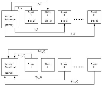
until (6) holds or jmax iterations are taken. Exceeding either iteration limit is a failure and causes the difference increment to be reduced. We set jmax=kmax=5 with a goal of taking barely enough iterations to resolve the solution. As for parallelism, 8 processors were used. One of the processors runs the IFFCO code (call it the master). The other 7 processors will evaluate f (call them the slaves). The master processor sends the values at which f must be evaluated to build the difference gradient to the 7 slave processors. The slave processors then send the evaluated functions back to the master processor. The master repeats this until all the needed points are evaluated and then the master processor computes the gradient. Figure 6 shows a general master-slave processor arrangement with k slaves evaluating the function at different points and one master that assembles the gradients and runs IFFCO.

Figure 6 Master-Slave Processor Arrangement

The language PVM [7] was used to handle the parallelism. PVM stands for Parallel Virtual Machine and allows communication between the different processors or computers. PVM is usually very portable. In this case though a T3D version of PVM was used. The reason it is not portable is due to a few specialized T3D commands, but this can easily be modified for non-T3D networks.

(6)

program on all of its processors. In our case it runs the valve code on all of its processors. Then when the valve code calls IFFCO, IFFCO must choose a master processor to run its code on. The other processors will be the slave processors. At that point the slaves go to a routine where they await instructions while the master executes IFFCO. Then when IFFCO calls the gradient evaluation routine, the code figures out ahead of time which points need to be evaluated (i.e. it figures out whether to evaluate a central, forward or backward difference for each component of the gradient). This simplifies the data handling because then are just a list of points need to be evaluated and sent back to the different processors. The processors send the data back to the master processor and then the master processor evaluates the appropriate differences accordingly and forms the gradient.

Because of the computationally intensive valve train simulation, the overhead in communication was a very small part of the overall computation. The 8 processor runs on the T3-D were over 20 times faster, in terms of wall-clock time, than similar computations on a 133MHz Pentium® machine.

PARAMETER IDENTIFICATION RESULTS

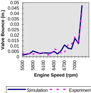
Figure 7 shows the results of a parameter identification for a typical racing valve train. Is show the predicted valve bounce and the measured valve bounce over a range of engine speeds. The agreement is quite good, and most importantly the instability speed is predicted quite accurately. This parameter identification took approximately 24 hrs on a 133 MHz Pentium® based computer and approximately 1 hr on the Cray T3D. Thus, the accuracy of the model is verified, along with the robustness of the optimizer and parallel computing algorithm.

OPTIMAL DESIGN

With an accurate model, the optimization process can begin. As this system has over 30 parameters, any or all of them could be optimized. In most mechanical system, several parameters are potential candidates for

optimization. However, for this system, many of the

0 0.005 0.01 0.015 0.02 0.025 0.03 0.035 0.04 0.045 0.05

5500 5800 6100 6400 6700 7000

Engine Speed (rpm)

Valve Bounce (in.)

Simulation Experiment

Figure 7 Comparison of Simulation with Experiment

parameters are determined by geometric and/or manufacturing parameters or engine operational constraints. In that the camshaft is the input forcing function, it was chosen as the focus of this optimization attempt. To this end, the camshaft lift curve was broken into segments as detailed in Park and David [8]. Fifteen nondimensional parameters were used to define the lift curve. The objective function for the optimal design portion of this study was

f

valve bounce

i nspeed

=

∑

(

_

)

2

1

(9) where valve_bounce is the amplitude of the first valve bounce after valve closure.

(7)

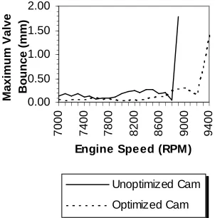
addition, the intermediate speed performance was improved as indicated by the reduction in valve bounce.

0.00 0.50 1.00 1.50 2.00

7000 7400 7800 8200 8600 9000 9400 Engine Speed (RPM) Maximum Valve Bounce (mm)

Unoptimized Cam

Optimized Cam

Figure 8 Optimal Design Results for a NASCAR Valve Train

Figure 9 shows the results of a design done for the Buick V-6 Indy Program in 1992. As before, the maximum cam lift and duration was identical between the two designs, but the optimal design produced a 300 rpm increase in engine speed and greatly improved the intermediate speed performance of the mechanism.

0 0.2 0.4 0.6 0.8 1

7000 7400 7800 8200 8600 9000 9400 9800 Engine Speed (rpm )

Maximum Valve Bounce

(mm)

Original Cam Optimized Cam

Figure 9 Optimal Design Results for the Buick V-6 Indy Engine

CONCLUSIONS

The strategy presented in this paper of

• modeling

• experimentation

• parameter identification

• optimal design

produced designs which significantly improved the performance of these high-speed mechanical systems. The use of a robust optimization algorithm in conjunction with a parallel processor produced results in reasonable times so as to be useful to machine designers. An important aspect of the process was developing a model which was computationally efficient as well as accurate, requiring a level of expertise of the engineer normally associated with the designer.

ACKNOWLEDGEMENTS

The authors gratefully acknowledge the support of Mr. Jim Covey and Mr. Bernard Santavy of the Motorsports Technology Group, General Motors Corporation for their support of the work of Drs. David and Cheng. In addition, the work of Dr. Kelley and Mr. Choi was supported by National Science Foundation grants DMS-9321938 and DMS-9700059 and the U. S. Department of Education GAANN fellowship. Computing activity was partially supported by an allocation from the North Carolina Supercomputing Center. The work of Mr. Gablonsky was supported by the International Student Exchange Program.

REFERENCES

[1] D. Kim, Dynamics and Optimal Design of High

Speed Valve Train Systems, Ph.D. thesis,

Mechanical and Aerospace Engineering, North Carolina State University, Raleigh, NC, 1990. [2] D. Kim and J.W. David, A Combined Model for

High-Speed Valve Train Dynamics, Partly Linear and Partly Nonlinear, SAE Technical Paper Series

901726.

[3] J.W. David, C.T. Kelley and C.Y. Cheng, Use of

an Implicit Filtering Algorighm for Mechanical System Parameter Identification, SAE Technical

(8)

[4] P. Gilmore and C.T. Kelley, An Implicit Filtering

Algorithm for Optimization of Functions with Many Local Minima, SIAM Journal of Optimization,

Vol. 5, No. 2, May, 1995

[5] D.B. Bertsekas, On the Goldstein-Levitin-Polyak

Gradient Projection Method, IEEE Transactions on

Automatic Control, 21 (1976), pp. 174-184.

[6] P. Gilmore and C.T. Kelley, An Implicit Filtering

Algorithm for Optimization of Functions with Many Local Minima, Tech. Report CRSC-TR94-23, North

Carolina State University, Center for Research in Scientific Computation, December, 1994.

[7] A. Geist, A. Beguelin, J. Dongarra, E. Jiang, R. Manchek, V. Sunderam. PVM: Parallel Virtual

Machine A Users' Guide and Tutorial for Networked Parallel Computing, MIT Press, 1994.

[8] Park, D.C. and J.W. David, “Development of a Locally Nondimensional, Mathematically Symmetric Cam Profile for Optimal Camshaft Design”, SAE