Multimodal Distributional Semantics

(1)

XXVI Cycle

Doctor of Philosophy

Multimodal distributional semantics

Elia Bruni

Advisors: Prof. Marco Baroni

(2)

Thesis Committee:

Marco Baroni, Thesis Advisor

Daniel Gatica-Perez

Sebastian Padó

(3)

(4)

(5)

(6)

Acknowledgements

The completion of my thesis and subsequent Ph.D. has been a won-derful adventure.

First of all, I am grateful to my advisor Marco Baroni for life. Working with you has been an illuminating experience. You have been a steady support throughout my Ph.D. career; you have always been patient but also motivating in times of difficulties. Above all, I have found a friend in you.

My sincere thanks to Google Inc. for having supported my Ph.D. with a Google Research Award assigned to Marco Baroni. Thanks to Massimiliano Ciaramita, for his unconditional support to my research. A very special thank goes to Jasper Uijlings, whose computer vision understanding is tremendous and whose scientific work has inspired me. My work has greatly benefited from your suggestions.

Another special thank goes to Claudio Martella, who patiently ex-plained me everything about programming.

Thank you to Roberto Zamparelli and Raffaella Bernardi for your support. Thanks to Leah Mercanti, the secretary that anyone would want to have!

I am also indebted to the students I had the pleasure to work with. You have been an invaluable help day in, day out, during all these years. Thanks to Giang Binh Tran, Nam Khan Tran, Ulisse Bor-dignon, Adam Liška and Irina Sergienya.

(7)

such a pleasant and productive working atmosphere. Thank you Moto for your delicious dinners! Thanks to Victoria Yanulevskaya, Gemma Boleda, Nicu Sebe, David Melcher, Francesca Bacci, Elisa Zamboni, Massimo Poesio and Andrew Anderson, it has been a pleasure to work with you.

A very big thank goes to Sebastian Petersson and Jacopo Amidei, who hosted me in Siena during the thesis write-up: It had been a really magic time!

(8)

(9)

Although being one very simple statement, the distributional hypoth-esis - namely, words that occur in similar contexts are semantically similar - has been granted the role of main assumption in many com-putational linguistic techniques. This is mostly due to the fact that it allows to easily and automatically construct a representation of word meaning from a large textual input.

Among the computational linguistic techniques that are corpus-based and adopt the distributional hypothesis, Distributional semantic mod-els (DSMs) have been shown to be a very effective method in many semantic-related tasks. DSMs approximate word meaning by vectors that keep track of the patterns of co-occurrence of words in the pro-cessed corpora. In addition, DSMs have been shown to be a very plausible computational model for human concept cognition, since they are able to simulate several psychological phenomena.

Despite their success, one of their strongest limitations is that they entirely represent word meaning in terms of connections with other words. Cognitive scientists have argued that, in this way, DSMs ne-glect that humans rely also on non-verbal experiences and have access to rich sources of perceptual knowledge when they learn the meaning of words.

(10)

(11)

List of Figures

3.1 Example results of the (left) Hessian detector; (right) Harris de-tector. [Figure from Krystian Mikolajczyk] . . . 21 3.2 Automatic scale selection: Given a keypoint location, a

scale-dependent signature function of the region around the keypoint is computed and the resulting value are plotted as a function of the scale. [Figure from Krystian Mikolajczyk] . . . 22 3.3 The Laplacian-of-Gaussian (LoG) detector searches for 3D scale

space extrema of the LoG function. [Figure from Krystian Miko-lajczyk] . . . 23 3.4 The SIFT descriptor. For each localized region, image gradients

are computed on a regular grid and then encoded into a 4×4 grid

of local gradient orientations (the figure shows only a 2×2 grid). . 24

3.5 Samples of images and their tags from the ESP-Game data set . . 28 3.6 The procedure to build an image-based semantic vector for a target

word. First, a bag-of-visual-word representation for each image labeled with the target word is computed (in this case, three images are labeled with the target word monkey). Then, the visual word occurrences across instance counts are summed to obtain the co-occurrence counts associated with the target word. . . 31

4.1 Multimodal fusion for combining textual and visual information in a semantic model. . . 39

(16)

LIST OF FIGURES

5.1 Distribution of z-normalized cosines of words instantiating vari-ous relations across BLESS pivots. Text-based vectors from the Window20 model. . . 52

6.1 Discrimination of literal (L) vs. nonliteral (N) uses by the best visual and textual models. . . 83

7.1 It is easier to distinguish the deer from the wolf once we local-ize them, but the surroundings tell us that they live in a similar environment, and are thus somewhat related concepts. . . 86 7.2 Similarity matrices for the human subjects. Lighter color cues

higher similarity. . . 89 7.3 Similarity matrices for Global. Lighter color cues higher similarity. 90 7.4 Similarity matrices for AL-Object. Lighter color cues higher

simi-larity. . . 91 7.5 Similarity matrices for AL-Context. Lighter color cues higher

sim-ilarity. . . 92 7.6 Similarity (Pearson correlation) between each category pair in

oc-cipital lobe. . . 105 7.7 Similarity (Pearson correlation) between each category pair in frontal

lobe. . . 106

9.1 An example of a visual vocabulary creation pipeline. From a set of images, a larger set of features are extracted and clustered, forming the visual vocabulary. . . 121 9.2 An example of a BoVW representation pipeline for an image.

Fig-ure inspired byChatfield et al.[2011]. Each feature extracted from the target image is assigned to the corresponding visual word(s). Then, spatial binning is performed. . . 122 9.3 An example of a concept representation pipeline for cat. First,

several images depicting a cat are represented as vectors of visual word counts and, second, the vectors are aggregated into one single concept vector. . . 123

(17)

List of Tables

5.1 Attributes preferred by text- (Window20) vs. image-based models. 53 5.2 Spearman correlation of the models on MEN and WordSim (all

coefficients significant with p < 0.001). TunedFL is the model automatically selected on the MEN development data. . . 58 5.3 Pearson correlation of some of our best multimodal combinations

on the WordSim subset covered by Feng and Lapata [2010] (all coefficients significant with p < 0.001; Pearson used instead of Spearman for full comparability with Feng and Lapata). The mod-els assigned 0 similarity to the 71/253 pairs for which they were missing a vector. Feng and Lapata [2010] report 0.32 correlation for MixLDA. . . 59 5.4 Top 10 pairs whose relatedness is better captured by Text

(Win-dow20) vs. TunedFL. . . 61 5.5 Percentage purities of the models on AP. TunedFL is the model

automatically selected on the Battig data . . . 65 5.6 Spearman correlation of the new models on MEN and WordSim353

(all coefficients significant with p <0.001). . . 67 5.7 Purity values of the new models on AP. . . 67 5.8 Top 10 closest words to the concrete words provided by the global

weighting model. . . 69 5.9 Top 10 closest words to the abstract words provided by the global

weighting model. . . 69 5.10 Top 10 closest words to the concrete words provided by the local

weighting model. . . 70

(18)

LIST OF TABLES

5.11 Top 10 closest words to the abstract words provided by the local weighting model. . . 70

6.1 Results of the textual, visual, multimodal, and hybrid models on the general semantic tasks (first two columns, section6.2; Pearson ρ) and Experiments 1 (E1, section 6.3) and 2 (E2, section 6.4). E1 reports the median rank of the correct color and the number of top matches (in parentheses), and E2 the average difference in normalized cosines between literal and nonliteral adjective-noun phrases, with the significance of a t-test (*** for p< 0.001, ** <0.01, * <0.05). . . 79

7.1 Percentage Spearman correlations of the models with human se-mantic relatedness intuitions for the Pascal concepts. . . 93 7.2 The 51 words represented by the brain and the distributional

mod-els, organized by category. . . 96 7.3 Matrix of correlations between each pairwise combination of

distri-butional semantic models and brain data. Correlations correspond to the pairwise similarity between the 11 categories. In each col-umn the first value corresponds to Spearman’s rank correlation coefficient and the value in parenthesis is the p-value. . . 103 7.4 Matrix of correlations between each pairwise combination of

distri-butional semantic models and brain data. Correlations correspond to the pairwise similarity between the 51 words. In each column the first value corresponds to Spearman’s rank correlation coeffi-cient and the value in parenthesis is the p-value. . . 103

(19)

Parts of this thesis (ideas, figures, results, and discussions) have been presented previously in the following publications:

Elia Bruni, Nam Khan Tran and Marco Baroni. Multimodal distri-butional semantics. Submitted.

Andrew Anderson, Elia Bruni, Ulisse Bordignon, Massimo Poesio and Marco Baroni. Of words, eyes and brains: Correlating image-based distributional semantic models with neural representations of concepts. In Proceedings of EMNLP 2013 (Conference on Empiri-cal Methods in Natural Language Processing), East Stroudsburg PA: ACL.

Elia Bruni, Ulisse Bordignon, Adam Liška, Jasper Uijlings, and Irina Sergienya. VSEM: An open library for visual semantics representa-tion. InProceedings of the 51st Annual Meeting of the Association for Computational Linguistics: System Demonstrations, pages 187–192, Sofia, Bulgaria, August 2013. Association for Computational Linguis-tics (ACL).

(20)

(21)

(22)

Chapter 1

Introduction

1.1

Semantic space models

Distributional semanticsis the branch of computational linguistics that devel-ops methods to approximate the meaning of words based on their distributional properties in large textual corpora. The basis of such methods relies on the distributional hypothesis: Words that occur in similar context are seman-tically similar. Although the distributional hypothesis has multiple theoretical underpinnings in psychology, linguistics, lexicography and philosophy of language [Firth, 1957; Harris, 1954; Miller and Charles, 1991; Wittgenstein, 1953], nowa-days its strong influence is mainly due to its practical consequence: Harvesting meaning becomes the very straightforward operation of recording the contexts in which words occur and using their co-occurrence statistics to represent their meanings. Distributional semantic models (DSMs) are among the approaches which take full advantage of the distributional hypothesis by storing distributional information into vectors that can be utilized to compute the degree of semantic relatedness of two or more words in terms of geometric distance (see e.g., Clark

[2013]; Turney and Pantel [2010]). For example, both sea and ocean might of-ten appear with words such as water, boat, fish and wave and, as a result, their distributional vectors will be very close, indicating that the two words are very similar. The way in which DSMs operationalize the distributional hypothesis has led to very effective approaches in many semantic-related tasks (see Section 2.1

(23)

for some references), also helping confirming the validity of the hypothesis.

1.2

The symbol grounding problem

Despite its great success, distributional semantics has the clear limitation of re-ducing the acquisition of word meaning solely to the linguistic input, ignoring other important channels of information such as the perceptual one. A long tra-dition of studies which goes from philosophy to cognitive science has developed a strong objection against models which represent the meaning of symbols (e.g., words) in terms of other symbols (e.g., other words) and without any connection to the outside world, called the symbol grounding problem [Harnad, 1990]. DSMs have also to be considered defective with respect of the symbol grounding problem and have come under attack for their lack of grounding [Glenberg and Robertson, 2000].

Although the specific criticisms vented at them might not be entirely well-founded [Burgess, 2000], there can be little doubt that the limitation to textual contexts makes DSMs very dissimilar from humans, who, thanks to their senses, have access to rich sources of perceptual knowledge when learning the meaning of words – so much so that some cognitive scientists have argued that meaning is directly embodied in sensory-motor processing (for different views on embod-iment in cognitive science de Vega et al. [2008]). Indeed, in the last decades a large amount of behavioural and neuroscientific evidence has been amassed indi-cating that our knowledge of words and concepts is inextricably linked with our perceptual and motor systems. For example, perceiving action-denoting verbs such as kick or lick involves the activation of areas of the brain controlling foot and tongue movements, respectively [Pulvermueller, 2005]. Hansen et al. [2006] asked subjects to adjust the color of fruit images objects until they appeared achromatic. The objects were generally adjusted until their color was shifted away from the subjects’ gray point in a direction opposite to the typical color of the fruit, e.g., bananas were shifted towards blue because subjects’ overcor-rected for their typical yellow color. Typical color also influences lexical access: For example, subjects are faster at naming a pumpkin in a picture in which it is presented in orange than in a grayscale representation, slowest if it is in

(24)

1. Introduction

other color [Therriault et al., 2009]. As a final example, Kaschak et al. [2005] found that subjects are slower at processing a sentence describing an action if the sentence is presented concurrently to a visual stimulus depicting motion in the opposite direction of that described (e.g., The car approached you is harder to process concurrently to the perception of motion away from you). See Barsalou

[2008] for a review of more evidence that conceptual and linguistic competence is strongly embodied.

One might argue that the concerns about DSMs not being grounded or em-bodied are exaggerated, because they overlook the fact that the patterns of lin-guistic co-occurrence exploited by DSMs reflect semantic knowledge we acquired through perception, so that linguistic and perceptual information are strongly correlated [Louwerse, 2011]. Because dogs are more often brown than pink, we are more likely to talk about brown dogs than pink dogs. Consequently, a child can learn useful facts about the meaning of the concept denoted by dog both by direct perception and through linguistic input (this explains, among other things, why congenitally blind subjects can have an excellent knowledge of color terms; see, e.g., Connolly et al. [2007]). One could then hypothesize that the meaning representations extracted from text corpora are indistinguishable from those derived from perception, making grounding redundant. However, there is by now a fairly extensive literature showing that this is not the case. Many stud-ies [Andrews et al., 2009; Baroni and Lenci, 2008; Baroni et al., 2010; Riordan and Jones, 2011] have underlined how text-derived DSMs capture encyclopedic, functional and discourse-related properties of word meanings, but tend to miss their concrete aspects. Intuitively, we might harvest from text the information that bananas are tropical and eatable, but not that they are yellow (because few authors will write down obvious statements such as “bananas are yellow”). On the other hand, the same studies show how, when humans are asked to describe concepts, the features they produce (equivalent in a sense to the contextual fea-tures exploited by DSMs) are preponderantly of a perceptual nature: Bananas are yellow, tigers have stripes, and so on.1

1_{To be perfectly fair, this tendency might in part be triggered by the fact that, when}

subjects are asked to describe concepts, they might be encouraged to focus on their perceptual aspects by the experimenters’ instructions. For example McRae et al.[2005] asked subjects to list first “physical properties, such as internal and external parts, and how [the object] looks.”

(25)

This discrepancy between DSMs and humans is not,per se, a proof that DSMs will face empirical difficulties as computational semantic models. However, if we are interested in the potential implications of DSMs as models of how humans acquire and use language –as is the case for many DSM developers [Griffiths et al., 2007; Landauer and Dumais, 1997; Lund and Burgess, 1996]– then their complete lack of grounding in perception is a serious blow to their psycholog-ical plausibility, and exposes them to all the criticism that classic ungrounded symbolic models have received. Even at the empirical level, it is reasonable to expect that DSMs enriched with perceptual information would outperform their purely textual counterparts: Useful computational semantic models must capture human semantic knowledge, and human semantic knowledge is strongly informed by perception.

If we accept that grounding DSMs into perception is a desirable avenue of research, we must ask where we can find a practical source of perceptual infor-mation to embed into DSMs. Several interesting recent experiments use features produced by human subjects in concept description tasks (so-called “semantic norms”) as a surrogate of true perceptual features [Andrews et al., 2009; Johns and Jones, 2012; Silberer and Lapata, 2012; Steyvers, 2010]. While this is a reasonable first step, and the integration methods proposed in these studies are quite sophisticated, using subject-produced features is unsatisfactory both practi-cally and theoretipracti-cally (see however for a crowdsourcing project that is addressing both kinds of concernsKievit-Kylar and Jones[2011]). Practically, using subject-generated properties limits experiments to those words that denote concepts de-scribed in semantic norms, and even large norms contain features for just a few hundred concepts. Theoretically, the features produced by subjects in concept description tasks are far removed from the sort of implicit perceptual features they are supposed to stand for. For example, since they are expressed in words, they are limited to what can be conveyed verbally. Moreover, subjects tend to produce only salient and distinctive properties. They do not state that dogs have a head, since that’s hardly a distinctive feature for an animal!

(26)

1. Introduction

1.3

The proposed approach

The work presented in this thesis aims at filling the gap between the automatically constructed distributional semantic models and the human semantic memory, by building new DSMs that are perceptually grounded. In particular, we exploit recent advances in image analysis to extract compact representation of meaning from pictures, by extracting co-occurrence counts of target words and visual col-locates from large datasets of tagged images. Thanks to these techniques, it is indeed possible to summarize an image by discretizing its content in vectors that keep track of visual unit counts. Moreover, we compose the obtained image-based DSMs with text-based DSMs and obtain multimodal representation of meaning.

1.4

Outline of the thesis

The main topic of this manuscript consists in the integration into DSMs of a more natural source of visual perceptual information (the relevant background from traditional and multimodal semantics is presented in Chapter2). We exploit recently introduced image analysis techniques which allow us to encode the visual information in a way that is compatible with standard text-based distributional models of semantics. More in the detail, as visual perceptual source, we use collections of images naturally co-occurring with words (i.e., words appear as tags describing the image content). As feature extraction pipeline, we exploit recent advances in computer vision that can be broadly divided into two main steps. First, we use algorithms which encode the image contents in terms of low-level features. Low-level features are indeed ubiquitous in computer vision since are capable of automatically detecting and describing the most salient parts of an image. In the second step, we use the low level features extracted at step one to induce a more abstract model based on the well-established bags-of-visual-words method to represent images. The bag-of-visual-bags-of-visual-words method has the great advantage of discretizing the image content into a fixed-dimensionality feature vector and is a key transformation for our multimodal semantic representation.

In Chapter3, Sections3.1and3.2, the entire visual feature extraction pipeline is described.

(27)

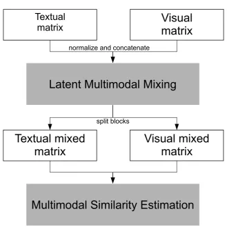
Processing an image collection via the visual pipeline sketched above is just the first step to obtain a multimodal distributional model. Once the visual features are extracted and they act as a purely image-based representation of meaning, they have to be integrated in a multimodal space where textual and visual seman-tic features can cohabit. Chapter 4is devoted exactly to this problem. The task of merging together two different channels of information can be pursued with increasingly sophisticated strategies. We will explore a first naive combination method that directly concatenates the visual and the textual vectors after a first normalization step (see Section 4.1). As an alternative, more advanced fusion strategy we propose a framework in which the textual and the visual features are projected into a common multidimensional space where they can interact, by promoting new connections between them (see Section 4.2). Moreover, in both Sections4.1 and4.2, each word in our framework is treated as requiring an equal amount of perceptual information, while it is natural to distinguish between very concrete, imageable words that require a fully perceptually informed feature rep-resentation, and abstract, non-imageable words, that are not “groundable" and therefore do not require perceptual features. Therefore, in Section4.3, we explore different measures and ways to incorporate them in a new concatenation system, which is able to model textual and visual feature fusion locally, at a word-by-word level.

Chapter 5 and Chapter 6 of the thesis address the evaluation of the pro-posed multimodal framework. Since there is not a unique test which is capable of measuring if and how visual features convey meaningful information into a distributional semantic model, we approach the evaluation problem from differ-ent angles. The core part of the evaluation is presdiffer-ented in Chapter 5. Here we conduct three different tests, one of which is qualitative in nature and tries to asses the overall pattern of semantic relations that the model is able to capture (Section 5.1), while the other two are quantitative analyses, testing the model on word relatedness tasks (Section 5.2 and 5.3). In the qualitative test we can spot some significant differences between a traditional text-based semantic model and an image-based semantic model, while in both the quantitative tests adding visual features to state-of-the-art textual features systematically augments the performance. The framework evaluation continues in Chapter 6, where, after

(28)

1. Introduction

double-checking the validity of an enlarged set of multimodal models on word relatedness, we tackle two tasks where visual information is highly relevant, as they focus on color. In the first task we try to discover the color of of 52 concrete objects. In the second task we try to discriminate between literal and nonlit-eral uses of color terms. We show that especially here visual information has a determinant role which leads to the absolute best performance both with visual features standalone and combined with textual features.

Chapter 7explores how information about object location can be used to ad-vance multimodal distributional semantics. In particular, in Section7.1we exploit location information to improve visual feature extraction to tackle a word relat-edness test. Interestingly, we show that a visual semantic model extracted only from within the precise location where the object appears in the image performs worse in the word relatedness task compared to a visual distributional model con-structed with the information coming from the surrounding of the object only. In Section 7.2, we test whether image-based models capture the semantic patterns that emerge from fMRI recordings of the neural signal. Our result show that there is indeed a significant correlation between image-based and brain-based se-mantic similarities, and that image-based models complement text-based models so that the best correlation are obtained when the two modalities are combined in a multimodal distributional model. Chapter8contains our conclusive remarks and future work about multimodal distributional semantics.

Finally, Appendix 9 introduces an off-the-shelf freely distributed library to build an image-based semantic model.

(29)

(30)

Chapter 2

Background

2.1

Distributional semantics

In the last few decades, a number of different distributional semantic models (DSMs) of word meaning have been proposed in computational linguistics, all relying on the assumption that word meaning can be learned directly from the linguistic environment.

Semantic space models are one of the most common types of DSM. They approximate the meaning of words with vectors that record their distributional history in a corpus[Turney and Pantel, 2010]. A distributional semantic model is encoded in a matrix whose m rows are semantic vectors representing the meanings of a set of m target words. Each component of a semantic vector is a function of the occurrence counts of the corresponding target word in a cer-tain context (see Lowe [2001], for a formal treatment). Definitions of context range from simple ones (such as documents or the occurrence of another word inside a fixed window from the target word) to more linguistically sophisticated ones (such as the occurrence of certain words connected to the target by special syntactic relations) [Padó and Lapata,2007; Sahlgren, 2005; Turney and Pantel,

2010]. After the raw target-context counts are collected, they are transformed intoassociation scoresthat typically discount the weights of components whose corresponding word-context pairs have a high probability of chance co-occurrence [Evert,2005]. The rank of the matrix containing the semantic vectors as rows can

(31)

optionally be decreased bydimensionality reduction, that might provide ben-eficial smoothing by getting rid of noise components and/or allow more efficient storage and computation [Landauer and Dumais,1997;Sahlgren, 2005;Schütze,

1997]. Finally, the distributional semantic similarity of a pair of target words is estimated by a similarity function that takes their semantic vectors as input and returns a scalar similarity score as output.

There are many different semantic space models in the literature. Proba-bly the best known is Latent Semantic Analysis (LSA, Landauer and Dumais

[1997]), where a high dimensional semantic space for words is derived by the use of co-occurrence information between words and the passages where they occur. Another well-known example is the Hyperspace Analog to Language model (HAL,

Lund and Burgess [1996]), where each word is represented by a vector containing weighted co-occurrence values of that word with the other words in a fixed win-dow. Other semantic space models rely on syntactic relations instead of windows [Curran and Moens,2002; Grefenstette,1994; Padó and Lapata, 2007]. For gen-eral overviews of semantic space models see Clark [2013]; Erk [2012]; Manning and Schütze [1999];Sahlgren [2006];Turney and Pantel [2010].

More recently, probabilistic topic models have been receiving increasing atten-tion as an alternative implementaatten-tion of DSMs [Blei et al., 2003; Griffiths et al.,

2007]. Probabilistic topic models also rely on co-occurrence information from large corpora to derive meaning but, differently from semantic space models, they are based on the assumption that words in a corpus exhibit some proba-bilistic structure connected to topics. Words are not represented as points in a high-dimensional space but as a probability distribution over a set of topics. Conversely, each topic can be defined as a probability distribution over different words. Probabilistic topic models solve the problem of meaning representation with a statistical inference: use the word corpus to infer the hidden topic struc-ture.

Distributional semantic models, whether of the geometric or the probabilis-tic kind, ultimately are mainly used to provide a similarity score for arbitrary pairs of words, and that is how we will also employ them. Indeed, such models have shown to be very effective in modeling a wide range of semantic tasks in-cluding judgments of semantic relatedness and word categorization [Almuhareb,

(32)

2. Background

2006;Baroni and Lenci,2010;Budanitsky and Hirst,2006;Radinsky et al.,2011;

Reisinger and Mooney, 2010;Rothenhäusler and Schütze,2009].

There are several data sets to assess how well a DSM captures human intu-itions about semantic relatedness, such as the Rubenstein and Goodenough set [Rubenstein and Goodenough, 1965] and WordSim353 [Finkelstein et al., 2002]. Usually they are constructed by asking subjects to rate a set of word pairs ac-cording to a similarity scale. Then, the average rating for each pair is taken as an estimate of the perceived relatedness between the words (e.g., dollar-buck: 9.22, cord-smile: 0.31). To measure how well a distributional model approximates human semantic intuitions, usually a correlation measure between the similarity scores generated by the model and the human ratings is computed. The highest correlation we are aware of on the WordSim353 set we will also employ below is of 0.80 and it was obtained by a purely textual model called Temporal Semantic Analysis, which captures patterns of word usage over time and where concepts are represented as time series over a corpus of temporally-ordered documents [Radinsky et al., 2011]. This temporal knowledge could be integrated with the perceptual knowledge we encode in our model.

Humans are very good at grouping together words (or the concepts they de-note) into classes based on their semantic relatedness [Murphy,2002], therefore a cognitive-aware representation of meaning must show its proficiency also in cat-egorization (e.g., Baroni et al. [2010]; Poesio and Almuhareb [2005]). Concept categorization is moreover useful for applications such as automated ontology construction and recognizing textual entailment. Unlike similarity ratings, cate-gorization requires a discrete decision to group coordinates/cohyponyms into the same class and it is performed by applying standard clustering techniques to the model-generated vectors representing the words to be categorized. An example of a categorization data set is the Almuhareb-Poesio [Almuhareb and Poesio, 2005] data set, that we we also employ below, and which includes 402 concepts from WordNet (see Section 5.3.1 below), balanced in terms of frequency and degree of ambiguity. Rothenhäusler and Schütze [2009] present a text-based approach that constitutes the state of the art on the Almuhareb-Poesio data set (maximum clustering purity: 0.79).

See Baroni and Lenci [2010] for a survey of other semantic tasks that DSMs

(33)

have been applied to, and Turney and Pantel [2010] for some of the applica-tions in which DSMs are employed, including document classification, clustering and retrieval, question answering, automatic thesaurus generation, word sense disambiguation, query expansion, textual advertising.

2.2

Multimodal distributional semantics

The availability of large amounts of mixed media on the Web, on the one hand, and the discrete representation of images as visual words on the other has not escaped the attention of computational linguists interested in enriching distribu-tional representations of word meaning with visual features.

Feng and Lapata[2010] propose the first multimodal distributional semantic model. Their generative probabilistic setting requires the extraction of textual and visual features from the same mixed-media corpus, because latent dimen-sions are here estimated through a probabilistic process which assumes that a document is generated by sampling both textual and visual words. Words are then represented by their distribution over a set of latent multimodal dimensions or “topics” [Griffiths et al., 2007] derived from the surface textual and visual fea-tures. Feng and Lapata experiment with a collection of documents downloaded from the BBC News website as corpus. They test their semantic representations on a subset of 254 pairs from the WordSim353 Word Similarity and Word Asso-ciation test collections, obtaining gains in performance for both test sets when visual information is taken into account (correlations with human judgments of 0.12 and 0.32 respectively), compared to the textual modality standalone (0.08 and 0.25 respectively), even if performance is still well below state-of-the-art for WordSim353 (see Section 2.1 above).

The main drawbacks of this approach are that the textual and visual data must be extracted from the same corpus, thus limiting the choice of the corpora to be used, and that the generative probabilistic approach, while elegant, does not allow much flexibility in how the two information channels are combined. Below, we re-implement the Feng and Lapata method (MixLDA) training it on the ESP-Game data set, the same source of labeled images we adopt for our model. This is possible because the data set contains both images and the textual

(34)

2. Background

labels describing them. More in general, we recapture Feng and Lapata’s idea of a common latent semantic space in the latent multimodal mixing step of our pipeline (see Section 5below).

Leong and Mihalcea[2011] also exploit textual and visual information to ob-tain a multimodal distributional semantic model. While Feng and Lapata merge the two sources of information by learning a joint semantic model, Leong and Mihalcea propose a strategy akin to what we will call Scoring Level fusion below: Come up with separate text- and image-based similarity estimates, and combine them to obtain the multimodal score. In particular, they use two combination methods: summing the scores and computing their harmonic mean. Differently fromFeng and Lapata[2010], here visual information for meaning representation is extracted not from a corpus but from a manually coded resource, namely the ImageNet1 _{database [}_{Deng et al.}_, ₂₀₀₉_{], a large-scale ontology of images. Using} a handcoded annotated visual resource such as ImageNet faces the same sort of problems that using a manually developed lexical database such as WordNet faces with respect to textual information, that is, applications will be severely limited by ImageNet coverage (for example, ImageNet is currently restricted to nominal concepts), and the interest of the model as a computational simulation of word meaning acquisition from naturally occurring language and visual data is somewhat reduced (humans do not learn the meaning of “mountain” from a set of carefully annotated images of mountains with little else crowding or occluding the scene). In the evaluation, Leong and Mihalcea experiment with small subsets of WordSim, obtaining some improvements, although not at the same level we re-port (the highest rere-ported correlation is 0.59 on just 56 word pairs). Furthermore they use the same data set to tune and test their models.

InBruni et al.[2011] we propose instead to directly concatenate the text- and image-based vectors to yield a single multimodal vector to represent words, as in what we call Feature Level fusion below. The text-based distributional vector representing a word, taken there from a state-of-the-art distributional semantic model [Baroni and Lenci, 2010], is concatenated with a vector representing the same word with visual features, extracted from all the images in the ESP Game collection we also use here. We obtain promising performance on WordSim and

1

http://image-net.org/

(35)

other test sets, although appreciably lower than the results we report here (we obtained a maximum correlation of 0.52 when text- and image-based features are used together; compare to Table5.2 below). Moreover, in Bruni et al.[2012a] we evaluate our multimodal models in the task of discovering the color of concrete objects, showing that the relation between words denoting concrete things and their typical color is better captured when visual information is also taken into account. Moreover, we show that multimodality helps in distinguishing literal and nonliteral uses of color terms.

Attempts to use multimodal models derived from text and images to perform more specific semantic tasks have also been reported. Bergsma and Goebel[2011] use textual and image-based cues to model selectional preferences of verbs (which nouns are likely arguments of verbs). Their experiment shows that in several cases visual information is more useful than text in this task. For example, by looking in textual corpora for words such as carillon, migas or mamey, not much useful information is obtained to guess which of the three is a plausible argument for the verb to eat. On the other hand, by exploiting Google image search functionality,1 enough images for these words are found that a vision-based model of edible things can classify them correctly.

Silberer and Lapata [2012] present a first survey about grounded models of semantic representation. The authors conduct a comparative study of semantic models that incorporate linguistic and perceptual information. They experiment with a model that combines the two different channels in a concatenated multi-modal space [Johns and Jones,2012] and with two joint models, which construct the multimodal representation from a joint distribution of the two channels [ An-drews et al., 2009] or from a joint “consensus" based on the correlation between the two channels [Hardoon et al., 2004]. They conclude that all models benefit form the integration of perceptual information since they obtain closer correspon-dence to human data, with a slightly better performance for the joint models. The novel comparative approach offers a nice and systematic overview of some fusion strategies in multimodal semantics. On the other hand, its main drawback is that the models under study cannot be really considered state-of-the-art mul-timodal representations. First, these models introduce perceptual information

1

http://images.google.com/

(36)

2. Background

with subject-produced features and not with more direct ways such as visual in-formation via image analysis, as in this paper. Second, their performance in the semantic tasks is well below state-of-the-art in the literature.

More recently,Silberer and Lapata[2013] show that visual attribute classifiers can act as an effective substitute for feature norms to physically ground word meaning. Describing images by their attributes is a very recent idea initially explored in works such as Ferrari and Zisserman [2007] and then successfully applied to object recognition starting from Farhadi et al. [2009]. Learning to describe images through their attributes allows to generalize to objects never seen before and even to transcend the category level, while providing a more general description of the visual input. Silberer and Lapata successfully applied visual attributes in multimodal distributional semantics, by first creating their own dataset of images and visual attributes for the nouns contained in theMcRae et al.

[2005] norms. Images were downloaded from ImageNet, while the a attributes were manually annotated by the authors. They proceeded by training a classifier for each attribute in their list. Each concept in their visual semantic space is then represented by a vector summarizing the attribute prediction scores of each image tagged with the target concept. They tested the resulting visual model standalone and combined with a purely textual model. As combination methods, they used a simple concatenation method and a more sophisticated approach based on Canonical Correlation Analysis [Hardoon et al., 2004]. Their results demonstrate that, compared to a purely textual (topic) model, visual attributes improve the performance of distributional models across different settings of a semantic association task based on the Nelson norms [Nelson et al., 1998]. In particular, the performance was improved by visual attributes either standalone or combined with the textual model.

2.3

Other work on combining text and image

data

Nowadays huge image collections are freely available on the Web, often incor-porating additional textual data such as tags, which provide complementary

(37)

formation related to the image content. The multimedia and computer vision communities have fruitfully used textual tags of image data to supplement im-age analysis and to help bridging the semantic gap that visual features alone cannot easily fill. Taking inspiration from methods originally used in text pro-cessing, algorithms for image labeling, search and retrieval have been built upon the connection between text and visual features. Barnard et al.[2003] present one of the first attempts to model multimodal sets of images with associated text, learning the joint distribution of image regions and concrete concepts. Their model has been recently extended to attributes such as yellow or striped [Berg

et al.,2010;Farhadi et al.,2009; Lampert et al.,2009;Wang and Forsyth,2009], enabling transfer learning to recognize attributes without hand-labeled training data [Farhadi et al.,2009; Lampert et al.,2009] and even unseen object recogni-tion by using a fast object localizarecogni-tion system which integrates addirecogni-tional proper-ties such as shape [Lampert et al., 2009]. Rohrbach et al.[2010] enhance transfer learning for attribute-based classification by using semantic relatedness values that they extract from textual knowledge bases.

The works reviewed above focus mostly on modeling the visual domain as opposed to the textual one, where, except forBerg et al.[2010], most use keywords rather than natural language captions. Both Farhadi et al. [2010] and Kulkarni et al. [2011] aim to associate more natural descriptions to images than just tags. They first use visual features to predict the content of an image in terms of objects and attributes. Then they use a natural language generation system to create image captions. Zha et al.[2009] present a system for visual query suggestion in image search. When users type a query, the system recommends them additional textual and visual queries that are semantically related with the original one in order to assist their searching process. Jamieson et al. [2010] propose an algorithm to simultaneously learn the names and the appearances of the objects represented in an unstructured collection of images containing a variety of objects within cluttered scenes.

Another interesting line of research exploits the connection between text and images with the goal to enhance human-robot interaction. For example,Chen and Mooney [2011] present an automatic system that understands natural-language navigation instructions by transforming them into an executable navigation plan.

(38)

2. Background

For the task, a semantic parser for interpreting the navigation instructions is learnt by observing how human followers act. Matuszek et al. [2012] present instead a model for grounded attribute learning. Using joint textual and visual information, they build a system capable of producing a set of (visual) attribute models that help in an object selection task. Given a set of objects G and a sentence such as “Here are the yellow ones,", the system (i.e., the robot) has to select only the yellow objects from G.

(39)

(40)

Chapter 3

Extraction of visual and textual

representations

In this Chapter we introduce the visual and the textual pipelines to construct image- and text-based distributional models respectively. Section 3.1 is entirely devoted to image processing. More in the detail, Section 3.1.1 introduces the means to obtain a first, low-level representation of the image content. Section 3.1.2 explains how to subsume such low-level information in a more abstract en-vironment, where the visual units are the extensively used visual words. Section 3.2 describes the actual image sources and parameters we utilized for our exper-iments. Section 3.3 provides all the specifications for the state-of-the-art textual models we used.

3.1

Extraction of visual features from images

This section overviews the recent advances in the field of image analysis. In particular, it introduces state-of-the-art algorithms to automatically produce a discrete representation of the image content. This is obtained in two main steps, namely by first encoding the image content in terms of local features and then by inducing a more abstract representation, based on the bag-of-visual-words technique.

(41)

3.1.1

Extraction of local features from images

In the last years, there has been a tremendous progress on the development of local features for analyzing images in order to tackle common computer vision tasks such as object recognition and image retrieval [Grauman and Leibe, 2011]. The key aspect which makes local features so effective is their invariance to a series of image transformations such as translation, rotation, scaling and affine deformation. Invariance is indeed at the basis of recognition and representation approaches which render them robust to a variety of viewing conditions, occlu-sions and image clutter.

A typical local feature extraction pipeline is composed of two steps: (i) Feature detection and (ii) Feature description. More details about each of the two phases follow.

3.1.1.1 Feature detection

Feature detection is the first important stage for local feature extraction, in which a set of distinctive keypoints are localized in the image. This is a delicate process because the detection of the selected keypoints must be repeatable under varying image conditions, viewpoint changes and the presence of noise. More technically, the extraction of the keypoints should produce the same feature coordinates no matter if the image is rotated or translated. Of course, not all points do satisfy these restrictive requirements. The motion of points lying on a uniform region is indeed not detectable since they are indistinguishable from its neighbors, while the motion ofpoints lying on a straight linecan be traced only if it is perpendicular to the line. Therefore, we are naturally led to consider points that exhibit signal changes in (at least) two directions as the proper candidates. In most of the cases these points happen to be corners: Imagine to examine the change of intensity in an image due to shifts in a local window; around a corner, the image intensity will change greatly as a local window is shifted in arbitrary directions.

Two common algorithms which implement these criteria are the Hessian de-tector [Beaudet,1978] and theHarris detector [Harris and Stephens,1988]1. The 1_{The list of feature detectors is not exhaustive. A much detailed discussion can be found}

in Mikolajczyk and Schmid[2005]

(42)

3. Extraction of visual and textual representations

Hessian detector looks at strong changes in two orthogonal directions and it is based on the matrix of the second derivatives of the image points, so-called Hes-sian. The points detected by this algorithm are mainly located on corners and in intensively textured areas. The Harris detector looks even more strictly at corners only. It proceeds by “searching for points x where the second-moment matrix C around x has two large eigenvalues” [Grauman and Leibe, 2011]. In Figure 3.1 the Harris responses are compared to those of the Hessian detector, showing that the former is slightly more accurate in individuating corners, while Harris returns also regions with strong textures.

20

CHAPTER 3. LOCAL FEATURES: DETECTION AND DESCRIPTION

Figure 3.7:

Example results of the (top left) Hessian detector; (top right) Harris detector;

(bottom left) Laplacian-of-Gaussian detector; (bottom right) Difference-of-Gaussian detector

(

IMAGE SOURCE: Krystian Mikolajczyk, bottom right image is from (Tuytelaars &

Mikola-jczyk 2007).

).

Since the scale coordinate is only sampled at discrete levels, it is important in

both the LoG and the DoG detector to interpolate the responses at neighboring scales

in order to increase the accuracy of detected keypoint locations. In the simplest version,

this could be done by fitting a second-order polynomial to each candidate point and its

two closest neighbors. A more exact approach was introduced by Brown & Lowe (2002).

This approach simultaneously interpolates both the location and scale coordinates of

detected peaks by fitting a 3D quadric function.

Finally, those regions are kept that pass a threshold

t

and whose estimated scale

falls into a certain scale range [s

min

, s

max

]. The resulting interest point operator reacts

to blob-like structures that have their maximal extent in a radius of approximately

1.6σ

of the detected points (as can be derived from the zero crossings of the modeled

Laplacian). In order to also capture some of the surrounding structure, the extracted

region is typically larger (most current interest region detectors choose a radius of

r

= 3σ

around the detected points). Figure 3.7(bottom right) shows the result regions

returned by the DoG detector on an example image. It can be seen that the obtained

regions are very similar to those of the LoG detector. In practice, the DoG detector is

therefore often the preferred choice, since it can be computed far more efficiently.

Figure 3.1: Example results of the (left) Hessian detector; (right) Harris detector. [Figure from Krystian Mikolajczyk]

While both the Hessian and the Harris detectors are exceptionally robust to image variations such as plane rotations, illumination changes and noise [Schmid et al., 2000], they still cannot offer locations which are robust enough to scale changes. If the location individuated by one of these detectors appear on a significantly larger scale within another image, the extracted structure will be different. This problem is due to the fact that both detectors utilize (Gaussian) derivatives computed on a single, fixed scale σ.

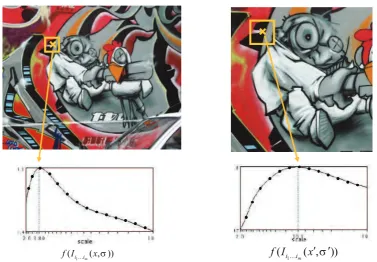
The solution consists in designing detection algorithms which become invari-ant to scale change by sampling the image at a range of scales (i.e., values of σ) automatically (see Figure 3.2).

(43)

16 CHAPTER 3. LOCAL FEATURES: DETECTION AND DESCRIPTION

)) , ( (I₁ xσ f i…i_m

)) , ( (

1 x′σ ′

I f

m i i…

Figure 3.3: The principle behind automatic scale selection. Given a keypoint location, we eval-uate a scale-dependent signature function on the keypoint neighborhood and plot the resulting value as a function of the scale. If the two keypoints correspond to the same structure, then their signature functions will take similar shapes and corresponding neighborhood sizes can be determined by searching for scale-space extrema of the signature function independently in both images. FIGURE FROM Krystian Mikolajczyk

principle, we could achieve this by sampling each image neighborhood at a range of

scales and performing

N

×

N

pairwise comparisons to find the best match. This is

however too expensive to be of practical use. Instead, we evaluate a

signature function

on each sampled image neighborhood and plot the result value as a function of the

neighborhood scale. Since the signature function measures properties of the local image

neighborhood at a certain radius, it should take a similar qualitative shape if the two

keypoints are centered on corresponding image structures. The only difference will be

that one function shape will be squashed or expanded compared to the other as a result

of the scaling factor between the two images. Thus, corresponding neighborhood sizes

can be detected by searching for extrema of the signature function

independently in both

images

. If corresponding extrema

σ

and

σ

!

are found in both cases, then the scaling

factor between the two images can be obtained as

σ! σ

.

Effectively, this procedure builds up a

scale space

(Witkin 1983) of the responses

produced by the application of a local kernel with varying scale parameter

σ

. In order

for this idea to work, the signature function or kernel needs to have certain specific

Figure 3.2: Automatic scale selection: Given a keypoint location, a scale-dependent signature function of the region around the keypoint is computed and the resulting value are plotted as a function of the scale. [Figure from Krystian Mikolajczyk]

One of the most utilized is the Laplacian-of-Gaussian LoG, which evaluates a scale-dependent signature function on the keypoint neighborhood and returns a value which is function of the scale [Lindeberg, 1998] (see Figure 3.3). One very popular version which approximates LoG is the Difference of Gaussians (DoG). DoG was introduced as the detection algorithm of the very popular feature descriptor Scale Invariant Feature Transform (SIFT), which we present below.

(44)

3. Extraction of visual and textual representations

18 CHAPTER 3. LOCAL FEATURES: DETECTION AND DESCRIPTION

) ( )

(σ _yyσ xx L

L +

σ σ2

σ3

σ4

σ5

Figure 3.5: The Laplacian-of-Gaussian (LoG) detector searches for 3D scale space extrema of the LoG function.Figure 3.3: The Laplacian-of-Gaussian (LoG) detector searches for 3D scale spaceIMAGE SOURCE: Krystian Mikolajczyk

extrema of the LoG function. [Figure from Krystian Mikolajczyk]

An additional step after having detected a scale-invariant region is that of normalizing the content for rotation invariance. The typical way to do it is by finding the region’s dominant direction and then by rotating the region content in accordance with this angle.

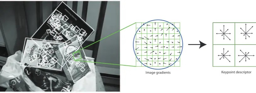
3.1.1.2 Feature description

Once a set of interesting regions is detected in an image by using one of the fea-ture detectors introduced above, their content has to be described and encoded in a suitable feature vector. This is done by a feature descriptor. The most pop-ular and effective descriptor is the Scale Invariant Feature Transform (SIFT), introduced by Lowe [1999, 2004]. As mentioned above, SIFT was originally in-troduced together with the DoG feature detector. Later, SIFT has been applied to other detectors such as Hessian, Harris and many more, achieving generally good performance as shown by Mikolajczyk and Schmid [2005]. More recently,

(45)

it has also been applied to dense grids (dense SIFT), which has been shown to yield better performance in tasks such as object recognition. Note that the dense SIFT is the solution that we also adopt.

The success obtained by SIFT is due to its robustness to variation of the image conditions such as lighting and small position shifts of the detected keypoints. In order to achieve such robustness, SIFT encodes the image information in a lo-calized set of gradient orientation histograms. The computation begins from one of the regions localized by one of the feature detectors (or by dense sampling). First of all, the image gradient magnitude and orientation is sampled around the keypoint location at a particular region scale. The sampling is computed on a 16×16 regular grid covering the region of interest. For each location, the gradient

orientation is stored into a smaller 4×4 subgrid of gradient orientation histograms

with 8 orientations bins each. Furthermore, each bin is weighted by the corre-sponding pixel’s gradient magnitude. Once all orientation histograms have been computed, the resulting entries are concatenated to form a single 4×4×8=128

dimensional feature vector. Figure 3.4 depicts this procedure for a smaller 2×2

grid.

24 CHAPTER 3. LOCAL FEATURES: DETECTION AND DESCRIPTION

Image gradients Keypoint descriptor

Figure 3.8: Visualization of the SIFT descriptor computation. For each (orientation-normalized) scale invariant region, image gradients are sampled in a regular grid and are then entered into a larger 4_×4 grid of local gradient orientation histograms (for visibility reasons, only a 2×2 grid is shown here).IMAGE SOURCE: DAVID LOWE.

Harris-Laplacian and Hessian-Laplacian detectors. Finally, we can further generalize those detectors to affine covariant region extraction, resulting in the Harris-Affine and

Hessian-Affinedetectors. The affine covariant region detectors are complemented by the

MSER detector, which is based on maximally stable segmentation regions. All of those detectors have been used in practical applications. Detailed experimental comparisons can be found in (Mikolajczyk & Schmid 2004, Tuytelaars & Mikolajczyk 2007).

3.3

LOCAL DESCRIPTORS

Once a set of interest regions has been extracted from an image, their content needs to be encoded in a descriptor that is suitable for discriminative matching. The most popular choice for this step is the SIFT descriptor (Lowe 2004), which we present in detail in the following.

3.3.1 THE SIFT DESCRIPTOR

The Scale Invariant Feature Transform (SIFT) was originally introduced by Lowe as combination of a DoG interest region detector and a corresponding feature descriptor (Lowe 1999, 2004). However, both components have since then also been used in isola-tion. In particular, a series of studies has confirmed that the SIFT descriptor is suitable for combination with all of the above-mentioned region detectors and that it achieves generally good performance (Mikolajczyk & Schmid 2005).

Figure 3.4: The SIFT descriptor. For each localized region, image gradients are computed on a regular grid and then encoded into a 4×4 grid of local gradient

orientations (the figure shows only a 2×2 grid).

A last step of normalization to unit length is performed, in order to adjust for

(46)

3. Extraction of visual and textual representations

image contrast.

3.1.2

Bag of visual words

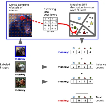
Ideally, to build a multimodal DSM, we would like to extract visual information from images in a way that is similar to how we do it for text. Thanks to a well-known image analysis technique, namely bag-of-visual-words (BoVW), it is indeed possible to discretize the image content and produce visual units somehow comparable to words in text, known asvisual words [Bosch et al.,2007;Csurka et al., 2004; Nister and Stewenius, 2006; Sivic and Zisserman, 2003; Yang et al.,

2007]. Therefore, semantic vectors can be extracted from a corpus of images associated with the target (textual) words using a similar pipeline to what is commonly used to construct text-based vectors: Collect co-occurrence counts of target words and discrete image-based contexts (visual words), and approximate the semantic relatedness of two words by a similarity function over the visual words representing them.

The BoVW technique to extract visual word representations of documents was inspired by the traditional bag-of-words (BoW) method in Information Retrieval. BoW in turn is a dictionary-based method to represent a (textual) document as a “bag” (i.e., order is not considered), which contains words from the dictionary. BoVW extends this idea to visual documents (namely images), describing them as a collection of discrete regions, capturing their appearance and ignoring their spatial structure (the visual equivalent of ignoring word order in text). A bag-of-visual-word representation of an image is convenient from an image-analysis point of view because it translates a usually large set of high-dimensional local features into a single sparse vector representation across images. Importantly, the size of the original set varies from image to image, while the bag-of-visual-word representation is of fixed dimensionality. Therefore, machine learning algorithms which by default expect fixed-dimensionality vectors as input (e.g., for supervised classification or unsupervised clustering) can be used to tackle typical image analysis tasks such as object recognition, image segmentation, video tracking, motion detection, etc.

More specifically, similarly to terms in a text document, an image has local

(47)

interest points or keypoints defined as salient image patches that contain rich local information about the image. However “keypoint types” in images do not come off-the-shelf like word types in text documents. Local interest points have to be grouped into types (i.e. visual words) within and across images, so that an image can be represented by the number of occurrences of each type in it, analogously to BoW. The following pipeline is typically followed. From every image of a data set, local features are extracted and represented as vectors as described in3.1.1. Feature vectors are then grouped across images into a number of clusters based on their similarity in descriptor space. Each cluster is treated as a discrete visual word. With its keypoints mapped onto visual words, each image can then be represented as a BoVW feature vector recording how many times each visual word occurs in it. In this way, we move from representing the image by a varying number of high-dimensional keypoint descriptor vectors to a representation in terms of a single visual word count vector of fixed dimensionality across all images, with the advantages we discussed above.

What kind of image content a visual word captures exactly depends on a num-ber of factors, including the descriptors used to identify and represent keypoints, the clustering algorithm and the number of target visual words selected. In gen-eral, local interest points assigned to the same visual word tend to be patches with similar low-level appearance; but these local patterns need not be correlated with object-level parts present in the images [Grauman and Leibe, 2011]. Vi-sual word assignment and its use to represent the image content is exemplified in Figure 1, where two images with a similar content are described in terms of bag-of-visual-word vectors.

3.2

Pipeline for visual representation

Given that image-based semantic vectors are a novelty with respect to text-based ones, in the next subsections we dedicate more space to how we constructed them, including full details about the source corpus we utilize as input of our pipeline (Section3.2.1), the particular image analysis technique we choose to extract visual collocates and how we finally arrange them into semantic vectors that constitute the visual block of our distributional semantic matrix (Section 3.2.2).

(48)

3. Extraction of visual and textual representations

3.2.1

Image source corpus

We adopt as our source corpus the ESP-Game data set1 _{that contains 100K} images, labeled through the famous “game with a purpose” developed by Louis von Ahn, in which two people partnered online must independently and rapidly agree on an appropriate word to label random selected images. Once a word is entered by both partners in a certain number of game rounds, that word is added as a tag for that image, and it becomes a taboo term for next rounds of the game involving the same image, to encourage players to produce more terms describing the image [Von Ahn, 2006]. The tags of images in the data set form a vocabulary of 20,515 distinct word types. Images have 14 tags on average (4.56 standard deviation), while a word is a tag for 70 images on average (737.71 standard deviation).

To have the words in the same format as in our text-based models, the tags are lemmatized and POS-tagged. To annotate the words with their parts of speech, we could not run a POS-tagger, since here words are out of context (i.e., each tag appears alphabetically within the small list of words labeling the same image and not within the ordinary sentence required by a POS-tagger). Thus we used a heuristic method, which assigned to the words in the ESP-Game vocabulary their most frequent tag in our textual corpora.

1

http://www.cs.cmu.edu/~biglou/resources/

(49)

Figure 3.5: Samples of images and their tags from the ESP-Game data set

The ESP-Game corpus is an interesting data set from our point of view since, on the one hand, it is rather large and we know that the tags it contains are re-lated to the images. On the other hand, it is not the product of experts labelling representative images, but of a noisy annotation process of often poor-quality or uninteresting images (e.g., logos) randomly downloaded from the Web. Thus, analogously to the characteristics of a textual corpus, our algorithms must be able to exploit large-scale statistical information, while being robust to noise. While cleaner and more illustrative examples of each concept are available in carefully constructed databases such as ImageNet (see Section 2.2), noisy tag annotations are available on a massive scale on sites such as Flickr1 _{and Facebook,}2 _{so if we} want to eventually exploit such data it is important that our methods can work on noisy input. A further advantage of ESP-Game with respect to ImageNet is that its images are associated not only with concrete noun categories but also

1

http://www.flickr.com

2

http://www.facebook.com

(50)

3. Extraction of visual and textual representations

with adjectives, verbs and nouns related to events (e.g., vacation, party, travel, etc). From a more practical point of view, “clean” data sets such as ImageNet are still relatively small, making experimentation with standard benchmarks dif-ficult. In concrete, looking at the benchmarks we experiment with, as of mid 2013, ImageNet covers only just about half the pairs in the WordSim353 test set, and less than 40% of the Almuhareb-Poesio words. While in the future we want to explore to what extent higher-quality data sources can improve image-based models, this will require larger databases, or benchmarks relying on a very restricted vocabulary.

The image samples in Figure3.5exemplify different kinds of noise that charac-terize the ESP-Game data set. Both on top and bottom left and top right there are images where the scene is cluttered or partially occluded. The top center image is hardly a good representative of accompanying words such as building, tower(s) or square. Similarly, the center bottom image is only partially a good illustration of a coin, and certainly not a very good example of a man! Finally, the bottom right image is useless from a visual feature extraction perspective.

3.2.2

Image-based semantic vector construction

We collect co-occurrence counts of target words and image-based contexts by adopting the BoVW pipeline that, as we already explained in Section 3.1.2, is particularly convenient in order to discretize visual information into “visual collo-cates”. We are adopting what is currently considered a standard implementation of BoVW. In the future, we could explore more cutting-edge ways to