Temperature Dependence of Kinetics for Reactive Diffusion in a Hypothetical Binary System

Temperature Dependence of Kinetics for Reactive Diffusion

in a Hypothetical Binary System

Masanori Kajihara

Department of Materials Science and Engineering, Tokyo Institute of Technology, Yokohama 226-8502, Japan

A hypothetical binary system consisting of two primary solid solution phases (and) and one compound phase () was considered in order to analyze theoretically the temperature dependence of kinetics for reactive diffusion. Assuming that migration of interface is controlled by volume diffusion in neighboring phases, the growth of thephase due to the reactive diffusion between theandphases in a semi-infinite diffusion couple was mathematically expressed as a function of the interdiffusion coefficients and the solubility ranges of the,andphases. The assumption yields that the square of the thicknesslof thephase is proportional to the annealing time taccording to the parabolic relationshipl2_{¼Kt, whereKis the parabolic coefficient. The present attention was focused on the relationship between the temperature} dependency of the growth rate and those of the interdiffusion coefficients, and hence the solubility ranges were assumed to be constant independently of the temperature and to take the same value for all the phases. On the contrary, the interdiffusion coefficientD_{(¼; ; ) was}

expressed as a function of the temperatureTby an Arrhenius equation ofD_¼D

0expðQ

_{=RTÞ. For simplicity, however,D}

0,D

0andD

0were considered equivalent. The temperature dependence of the parabolic coefficient K was described also by an Arrhenius equation of K¼K0expðQK=RTÞ, and thenK0andQKwere evaluated for various combinations ofQ,QandQ. The evaluation yields thatQKis equal to Q_{atQ¼Q¼Qand close toQatQQandQQ. Under such conditions, the temperature dependence ofDis estimated directly}

from that ofK. On the other hand,QKis greater thanQatQ>QorQ>Q. In this case, such estimation becomes invalid.

(Received July 25, 2005; Accepted August 26, 2005; Published October 15, 2005)

Keywords: intermetallic compounds, bulk diffusion, analytical methods, reactive diffusion, kinetics

1. Introduction

There exist many binary alloy systems where intermetallic compounds appear as stable phases.1)If a diffusion couple is prepared from two different pure metals in such a binary system and then annealed at an appropriate temperature T, some of the compounds may be recognized to form as layers at the interface between the two metals after certain periods due to reactive diffusion. Kinetics of the reactive diffusion was experimentally studied by many investigators for various alloy systems.2–20)_{When the reactive diffusion is controlled} by volume diffusion, the total thicknessl of the compound layers is described as a function of the annealing timet by the parabolic relationship l2_{¼Kt. Here,K is the parabolic}

coefficient. The temperature dependence of K may be ex-pressed by an Arrhenius equation ofK¼K0expðQK=RTÞ,

whereRis the gas constant. From experimental values ofKat different annealing temperatures, the pre-exponential factor K0and the activation enthalpyQK can be determined by the least-squares method. Most of the experimental studies indicate that the temperature dependence ofKis reasonably described by the Arrhenius equation within experimental uncertainty.2–20) _{Thus, it is expected that the Arrhenius} equation of K derives representative properties of the interdiffusion in the diffusion couple. However, K0 andQK contain complex information of the temperature depend-encies of the diffusion coefficients and the solubility ranges of the relevant phases. Consequently, such derivation is not so straightforward.

Recently, the reactive diffusion controlled by volume diffusion was theoretically analyzed by the present author using a mathematical model.21)In the theoretical analysis, a hypothetical binary alloy system composed of two primary solid solution phases and one intermetallic compound was

considered, and then the growth rate of the compound was evaluated for various semi-infinite diffusion couples initially consisting of the two primary solid solution phases. The mathematical model was also used to analyze numeri-cally the relationship between the temperature dependence of the interdiffusion in each phase and the kinetics of the reactive diffusion.22)_{In the numerical analysis, the} interdif-fusion coefficient D was described as a function of the annealing temperature T by an Arrhenius equation of D¼ D0expðQ=RTÞ, and the following assumptions were

adopt-ed: (a) the molar volume, the solubility range and the pre-exponential factorD0are constant and equivalent for all the

phases; and (b) the activation enthalpyQis equivalent for the solution phases but different between the solution phase and the compound. The numerical analysis indicates that the equationK¼K0expðQK=RTÞis reliable enough to express

the temperature dependence of experimental values ofKbut not necessarily completely exact. If Q is smaller for the compound than for the solution phases,QKis nearly equal to

Q of the compound. In such a case, the temperature dependence of K corresponds well with that of D of the compound. This relationship cannot hold good any longer, if Qis greater for the compound than for the solution phases. In order to examine whether such conclusions are universally valid, assumption (b) was eliminated for numerical analysis in a previous study.23)_{However, only limited combinations of} Qwere treated between the two solution phases, and thus the validity could not be confirmed conclusively. In the present study, similar numerical analysis has been carried out extensively for various combinations of Q among all the phases. Nevertheless, attention is still focused on the relationship between the temperature dependency of the kinetics and those of the interdiffusion coefficients of the constituent phases. Therefore, assumption (a) still remains for the numerical analysis in the present study.

*_{E-mail: [email protected]}

2. Analysis

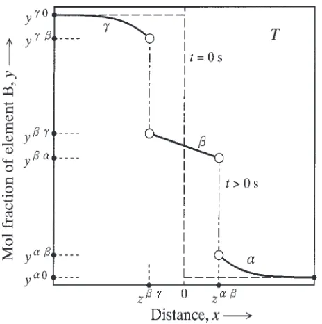
A hypothetical binary A–B system composed of two primary solid solution phases and one intermetallic com-pound was adopted in previous studies.21–23)_{The same binary} system was treated also in the present study. The and phases are the primary solid solution phases of elements A and B, respectively, and thephase is the compound. For the analysis, we consider a semi-infinite diffusion couple consisting of theandphases with initial compositions of y0 and y0, respectively. Here, y is the mol fraction of element B. In the semi-infinite diffusion couple, the thickness is semi-infinite for theandphases, and the=interface is flat. Therefore, the interdiffusion of elements A and B takes place unidirectionally along the direction perpendicular to the flat interface. This direction is hereafter called the diffusional direction. When the diffusion couple is annealed at temperatureT for an appropriate time, thephase will be produced as a layer at the interface due to the reactive diffusion between the and phases. The concentration profile of element B across the phase layer along the diffusional direction is schematically shown in Fig. 1.21) In this figure, the ordinate indicates the mol fraction y, and the abscissa shows the distancexmeasured from the initial position of the=interface. Dashed lines and solid curves indicate the concentration profiles before and after annealing, respectively, andz andz show the positions of the= and=interfaces, respectively, after annealing. If the local equilibrium is established at each migrating interface during annealing, the compositions of the neighboring phases at the interface coincide with those of the corresponding phase boundaries at temperature T in the phase diagram of the binary A–B system. As a result, the migration of the interface is controlled by the volume diffusion in the neighboring phases. In Fig. 1,y _{andy are the compositions of the} andphases, respectively, at the=interface, andy _and

yare those of theand phases, respectively, at the= interface. The compositionsy_{,y,y andyprovide the} boundary conditions, and those y0 _{and y}0 _{give the initial}

conditions.

If the reactive diffusion is controlled by the volume diffusion, the positions z _{and z of the = and =} interfaces are expressed as functions of the annealing timet by the equations

z¼Kpffiffiffiffiffiffiffiffiffiffi4D_t¼K ffiffiffiffiffiffiffiffiffiffi 4D_t p

ð1aÞ

and

z ¼Kpffiffiffiffiffiffiffiffiffiffi4D_t¼Kpffiffiffiffiffiffiffiffiffiffi_{4Dt; ð1bÞ}

respectively.24)Here, D, D and D are the interdiffusion coefficients for volume diffusion in the , and phases, respectively, and K,K,K andKare dimensionless coefficients. The thicknessl of the phase layer is readily obtained as the difference betweenz_{andz, and hence the} following equation is deduced from eq. (1) to expresslas a function oft.

l2¼ ðzzÞ2¼4DðKKÞ2t¼Kt ð2Þ

Here,Kis the parabolic coefficient defined as

K4DðKKÞ2: ð3Þ

The dimensionless coefficients are related to the initial and boundary conditions as follows:

cc¼ c 0_c

Kpffiffiffi_f1erfðKÞgexpfðK

Þ2g

þ c

_c

Kpffiffiffi_{ferfðKÞ erfðKÞg}

expfðKÞ2g ð4aÞ

and

cc ¼ c

_c

Kpffiffiffi_{ferfðKÞ erfðKÞg}expfðK _Þ2_g

þ c

0_c

Kpffiffiffi_{f1þerfðKÞg}expfðK

_Þ2_{g: ð4bÞ}

Here,cis the concentration of element B measured in mol per unit volume. The initial and boundary conditions are shown with the concentrationcin eq. (4), but indicated with the mol fractionyin Fig. 1. However,yis readily converted into c by the equation c¼y=Vm, where Vm is the molar volume of the relevant phase. The following relationships are obtained from eq. (1):

K¼KpffiffiffiffiffiffiffiffiffiffiffiffiffiffiD_{=D ð5aÞ}

and

K¼KpffiffiffiffiffiffiffiffiffiffiffiffiffiffiD_{=D: ð5bÞ}

Equation (5) shows that only two of the four dimensionless coefficients are independent. In the present analysis,K_and K _{are chosen as the independent variables. Insertion of} eq. (5) into eq. (4) yields two independent equations. Con-sequently, the two independent variables are finally deter-mined from the two independent equations.

3. Results and Discussion

Equations (2) to (5) indicate that the growth rate of the compound layer is controlled by the solubility ranges and the interdiffusion coefficients of the constituent phases in the diffusion couple. Hence, there are many parameters to determine the growth rate. As already mentioned in Section 1, however, the attention is focused on the relationship between the temperature dependency of the growth rate and those of the interdiffusion coefficients. Thus, in the present analysis, the solubility ranges of all the phases are considered constant independently of the temperature. Furthermore, it is assumed that the molar volume Vm is independent of the composition and equivalent for all the phases. According to this assumption, the concentrationsc0,c,c,c,cand c0 in eq. (4) are automatically replaced with the mol fractions y0_{, y, y, y, y and y}0_{, respectively. The}

following initial and boundary conditions are adopted in the present analysis:y0_{¼0,y¼0:1,y¼0:45,y ¼0:55,} y_¼0:9andy0_{¼1. Hence, independently of the}

temper-ature, the solubility rangeyis equal to 0.1 for all the phases, and the mean compositiony_{of the compound is identical to} 0.5: y¼y_y0_¼yy¼y0_{y¼0:1; and} y_{¼ ðyþyÞ=2¼0:5. The temperature dependence of} the interdiffusion coefficientDis described by the equation D¼D0expðQ=RTÞ. Here,D0is the pre-exponential factor,

andQis the activation enthalpy. The values ofQ,QandQ are varied from 50 to 100 kJ/mol, whereas the same value of D0¼104m2/s is used for all the phases in order to simplify

the analysis. Using these parameters, the parabolic coefficient K was numerically calculated as a function of T from eqs. (3)–(5) at a range ofT¼700{1000K. The temperature dependence of K was expressed by the equation K¼K0expðQK=RTÞ, and the pre-exponential factor K0

and the activation enthalpyQKwere determined in a manner similar to previous studies.22,23)

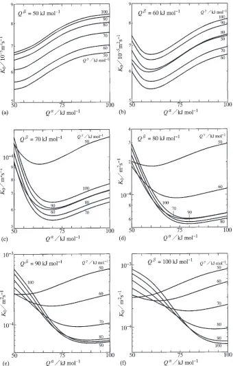
On the basis of the determination, dependencies ofK0 on

Q _{and Q were evaluated for various values of Q. The} results are shown as solid curves with constant values of Q _{¼50{100kJ/mol in Fig. 2. In this figure, the abscissa} indicates Q, and the ordinate shows the logarithm of K0.

Figures 2(a), (b), (c), (d), (e) and (f) indicate the evaluations forQ¼50, 60, 70, 80, 90 and 100 kJ/mol, respectively. At Q¼50kJ/mol in Fig. 2(a), K0 monotonically increases

with increasing value ofQ for each solid curve. For all the phases, the solubility rangeyand the pre-exponential factor D0 are identical to 0.1 and 104m2/s, respectively, as

mentioned earlier. Furthermore, the mean compositiony_of the compound is equal to 0.5. Thus, the effects ofQ_andQ on the temperature dependence of K are equivalent each other. As a result, K0 monotonically increases also with

increasing value ofQ_{at a constant value ofQ. On the other} hand, atQ_{¼60kJ/mol in Fig. 2(b),K}

0 slightly decreases

with increasing value ofQ_{, and reaches the minimum value} at Q¼60kJ/mol. After taking the minimum value, K0

gradually increases with increasing value ofQ. Due to the equivalence between the effects of Q and Q on the temperature dependence of K, the appearance of the mini-mum point is also the reason whyK0 is smaller for the solid

curves withQ _{¼60and 70 kJ/mol than for those withQ ¼}

50 and 80 kJ/mol but greater for those withQ ¼90 and 100 kJ/mol than for those withQ _{¼50and 80 kJ/mol. At} Q_{¼70kJ/mol in Fig. 2(c), however, the minimum point} shifts to Q

¼

_{70kJ/mol for the solid curves with Q ¼} 60{100kJ/mol, but almost stays atQ

¼

_{60kJ/mol for that} withQ _{¼50kJ/mol. On the contrary, atQ¼80kJ/mol in} Fig. 2(d), the minimum point nearly remains atQ_¼60and 70 kJ/mol for the solid curves withQ _{¼50and 60 kJ/mol,} respectively, but relocates toQ_{¼80kJ/mol for those with} Q _{¼70{100kJ/mol. In the case of Q¼100kJ/mol, K}

0

increases with increasing value ofQatQ¼50kJ/mol, but decreases with increasing value ofQ atQ¼100kJ/mol. Consequently, K0 varies depending on Q and Q in a

complicated manner as shown in Fig. 2(f).

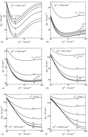
For various values ofQ, dependencies ofQK onQand

Q were evaluated together with those ofK0 onQandQ.

The results are indicated as solid curves with constant values of Q _{¼50{100kJ/mol in Fig. 3. The evaluations for} Q_{¼50, 60, 70, 80, 90 and 100 kJ/mol are shown in} Figs. 3(a), (b), (c), (d), (e) and (f), respectively. Figures 3(a) and (f) represent the results obtained in a previous study.23) At Q_{¼50kJ/mol in Fig. 3(a), Q}

K lightly decreases with increasing value of Q_{, and attains the minimum value at} Q_{¼60kJ/mol. After attaining the minimum value, Q}

K gradually increases with increasing value of Q_{. However,} such variations ofQKare rather small, and thusQKis close to

Q. On the other hand, atQ¼60kJ/mol in Fig. 3(b), the minimum point migrates toQ¼70kJ/mol for all the solid curves. QK is close to Q at Q¼60{100kJ/mol and

Q ¼60{100kJ/mol, but slightly greater than Q at Q_{¼50kJ/mol orQ ¼50kJ/mol. It is interesting to note} that the minimum point of the solid curve appears at different values of Q _{for K}

0 and QK as indicated in Figs. 2(b) and 3(b). According to the results in Figs. 3(c)–(f),QKis close to

Q _{at Q¼70{100kJ/mol and Q ¼70{100kJ/mol for} Q_{¼70kJ/mol, atQ¼80{100kJ/mol and Q ¼80{100} kJ/mol for Q_{¼80kJ/mol, at Q¼90{100kJ/mol and} Q _{¼90{100kJ/mol forQ¼90kJ/mol, and atQ¼100} kJ/mol and Q _{¼100kJ/mol for Q¼100kJ/mol.} How-ever,QK is greater thanQatQ¼50{60kJ/mol orQ ¼

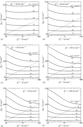
50{60kJ/mol forQ¼70kJ/mol, atQ¼50{70kJ/mol or Q ¼50{70kJ/mol forQ¼80kJ/mol, atQ¼50{80kJ/ mol or Q¼50{80kJ/mol for Q¼90kJ/mol, and at Q¼50{90kJ/mol or Q ¼50{90kJ/mol for Q¼100 kJ/mol. Thus, it is concluded thatQK is close toQatQ

Q_{andQ Qbut greater thanQatQ<QorQ <Q.} The results in Fig. 3 are shown in a different manner in Fig. 4. In this figure, solid curves indicate the evaluations with constant values of Q_{¼50{100kJ/mol. Open circles} show values of QK at Q¼Q, and a dashed straight line indicates a relationship of QK¼Q. Figures 4(a), (b), (c), (d), (e) and (f) show the results forQ _{¼50, 60, 70, 80, 90} and 100 kJ/mol, respectively. The results in Figs. 4(a) and (f) were reported in a previous study.23)_{AtQ ¼50kJ/mol in} Fig. 4(a),QKis rather insensitive to the variation ofQ, and close to Q for the solid curve with Q¼50kJ/mol. The open circle of this solid curve lies on the dashed line. However, QK is greater than Q for the solid curves with

the other hand, atQ _{¼60kJ/mol in Fig. 4(b),Q}

Kis close to

Q _{atQ50kJ/mol for the solid curve withQ¼50kJ/} mol and at Q_{60kJ/mol for that with Q¼60kJ/mol,} but slightly greater thanQ_{atQ<60kJ/mol for the latter} solid curve. The open circle of the solid curve with Q_¼ 60kJ/mol is completely located on the dashed line, but that of the solid curve with Q¼50kJ/mol lies slightly below the dashed line. For the solid curves withQ¼70{100kJ/ mol, however, QK is greater than Q. As can be seen in Figs. 4(c)–(f), QK is nearly equal to Q at QQ for

Q¼50{70kJ/mol atQ ¼70kJ/mol, forQ¼50{80kJ/

mol atQ _{¼80kJ/mol, forQ¼50{90kJ/mol atQ ¼90} kJ/mol and for Q_{¼50{100kJ/mol at Q ¼100kJ/mol.} For such combinations ofQ_{andQ, however,Q}

Kis greater thanQ_{atQ<Q. On the contrary, independently ofQ,} QK is greater thanQ for Q¼80{100kJ/mol atQ ¼70 kJ/mol, forQ¼90{100kJ/mol atQ ¼80kJ/mol and for Q¼100kJ/mol at Q ¼90kJ/mol. These relationships indicate that QK is close to Q at QQ for QQ. If such conditions are not realized, QK becomes greater thanQ.

From the evaluations in Fig. 3, the dependence of QK

Fig. 2 Dependencies ofK0 onQ andQ for (a)Q¼50kJ/mol, (b)Q¼60kJ/mol, (c)Q¼70kJ/mol, (d)Q¼80kJ/mol, (e)Q

¼90kJ/mol and (f)Q

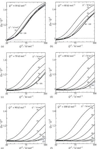
on Q _{is illustrated for various values of Q andQ. The} results with constant values of Q _{¼50{100kJ/mol are} shown as solid curves in Fig. 5. In this figure, the abscissa indicates Q_{, and the ordinate shows the ratio ofQ}

K toQ. Open circles indicate values of the ratioQK=Q_atQ¼Q, and a horizontal dashed line shows a value ofQK=Q¼1. The evaluations forQ¼50, 60, 70, 80, 90 and 100 kJ/mol are indicated in Figs. 5(a), (b), (c), (d), (e) and (f), respectively. At Q¼50kJ/mol in Fig. 5(a), the ratio QK=Q is equal to unity at Q¼50kJ/mol for the solid curve with Q ¼50kJ/mol, and close to unity at Q¼

50kJ/mol for those with Q_{¼60{100kJ/mol. As Q} increases, the ratio QK=Q _{monotonically increases, and} becomes greater for Q _{¼50kJ/mol than for Q ¼} 60{100kJ/mol. On the other hand, at Q_{¼60kJ/mol in} Fig. 5(b), the ratioQK=Q is equal to unity at Q¼60kJ/ mol forQ ¼60kJ/mol, and close to unity atQ60kJ/ mol forQ ¼70{100kJ/mol. Although the ratioQK=Qfor

Q ¼60kJ/mol is still smaller than that forQ ¼50kJ/mol, it becomes greater than that for Q ¼70{100kJ/mol at Q>60kJ/mol. At Q¼70kJ/mol in Fig. 5(c), the ratio QK=Qis equal to unity atQ¼70forQ ¼70kJ/mol, and

Fig. 3 Dependencies ofQKonQand Q for (a)Q¼50kJ/mol, (b)Q¼60kJ/mol, (c)Q¼70kJ/mol, (d)Q¼80kJ/mol,

close to unity at Q_{¼50kJ/mol for Q ¼50kJ/mol, at} Q_{60kJ/mol forQ ¼60kJ/mol and atQ70kJ/mol} for Q_{¼70{100kJ/mol. In the case ofQ¼80kJ/mol in} Fig. 5(d), however, the ratioQK=Qis equal to unity atQ¼

80forQ _{¼80kJ/mol, and close to unity atQ80kJ/mol} for Q _{¼90{100kJ/mol as well as at Q¼50kJ/mol for} Q ¼50kJ/mol, atQ60kJ/mol forQ ¼60kJ/mol and at Q70kJ/mol for Q¼70kJ/mol. Considering the results atQ¼90and 100 kJ/mol in Figs. 5(e) and (f), it is finally concluded that QK is exactly equal to Q at Q¼

Q¼Q and close toQ atQQ andQQ. Under such conditions, the activation enthalpy of the interdiffusion

coefficient in the growing compound layer is estimated directly from that of the parabolic coefficient. On the other hand,QK is greater thanQatQ>QorQ>Q. In this case, such estimation becomes invalid.

The reactive diffusion was experimentally studied for many binary systems consisting of elements with consider-ably different melting temperatures.10–20)When the melting temperature is much higher for thephase than for theand phases, the interdiffusion occurs much slower in the former phase than in the latter phases at a constant annealing temperature. Furthermore, the stable crystal structure of a compound is usually an ordered lattice in many binary

Fig. 4 Dependencies ofQKonQand Q for (a)Q¼50kJ/mol, (b)Q¼60kJ/mol, (c)Q¼70kJ/mol, (d)Q¼80kJ/mol,

systems.1)_{Thus, the interdiffusion in the phase should be} more sluggish than that in the phase unless the melting temperature is much lower for the phase than for the phase. Under such conditions, we may expect Q_> Q_{>Q. According to the conclusions mentioned above,} the temperature dependence of the interdiffusion coefficient in thephase cannot be estimated directly from that of the parabolic coefficient atQ>Q>Q. In this case, exper-imental information on the interdiffusion is essentially important for reliable estimation of the activation enthalpy of the interdiffusion coefficient in the compound.

4. Conclusions

The temperature dependence of the kinetics of reactive diffusion was theoretically analyzed for the hypothetical binary system composed of one compound phase () and two primary solid solution phases ( and ). The growth rate of the phase during the reactive diffusion between the and phases in a semi-infinite diffusion couple was expressed as a function of the interdiffusion coefficients and the solubility ranges of the , and phases using the mathematical model reported in a previous study.21) For simplicity, however, the solubility ranges of all the

Fig. 5 Dependencies of the ratioQK=Q_{onQandQfor (a)Q}

¼50kJ/mol, (b)Q

¼60kJ/mol, (c)Q

¼70kJ/mol, (d)Q

phases were assumed to be constant and equivalent. On the contrary, the interdiffusion coefficientD_{was described} as a function of the temperature T by the equation D_¼ D

0expðQ=RTÞ. Here,D0is the pre-exponential factor,Q

is the activation enthalpy,Ris the gas constant, andstands for , and . Furthermore, we assumed D

0 ¼D

0 ¼D

0.

For the reactive diffusion controlled by the volume diffusion, the square of the thicknesslof thephase is proportional to the annealing timetasl2_{¼Kt. The temperature dependence}

of the parabolic coefficientKwas expressed by the equation of K¼K0expðQK=RTÞ, and then the pre-exponential

factor K0 and the activation enthalpy QK were evaluated for different combinations of Q, Q and Q. In the case ofQ¼Q¼Q,QKis exactly equal toQ.QKis still close to Q at QQ and QQ. Under such conditions, the temperature dependence ofDis estimated directly from that ofK. Unfortunately, however,QKbecomes greater than

Q _{at Q>Q or Q>Q. In such a case, Q cannot} be estimated directly fromQK.

Acknowledgements

The present study was supported by a Grant-in-Aid for Scientific Research from the Ministry of Education, Culture, Sports, Science and Technology of Japan.

REFERENCES

1) T. B. Massalski, H. Okamoto, P. R. Subramanian and L. Kacprzak:

Binary Alloy Phase Diagram (ASM International, Materials Park, OH, 1990) vol. 1–3.

2) B. Lustman and R. F. Mehl: Trans. Met. Soc. AIME147(1942) 369– 394.

3) D. Horstmann: Stahl Eisen73(1953) 659–665.

4) S. Storchheim, J. L. Zambrow and H. H. Hausner: Trans. Met. Soc. AIME200(1954) 269–274.

5) G. V. Kidson and G. D. Miller: J. Nucl. Mater.12(1964) 61–69. 6) K. Shibata, S. Morozumi and S. Koda: J. Jpn. Inst. Met.30(1966) 382–

388.

7) K. Hirano and Y. Ipposhi: J. Jpn. Inst. Met.32(1968) 815–821. 8) M. M. P. Janssen: Metall. Trans.4(1973) 1623–1633.

9) G. F. Bastin and G. D. Rieck: Metall. Trans.5(1974) 1817–1826. 10) M. Onishi and H. Fujibuchi: Trans. JIM16(1975) 539–547. 11) EI-B. Hannech and C. R. Hall: Mater. Sci. Tech.8(1992) 817–824. 12) P. T. Vianco, P. F. Hlava and A. L. Kilgo: J. Electron. Mater.23(1994)

583–594.

13) M. Watanabe, Z. Horita and M. Nemoto: Interface Science4(1997) 229–241

14) S. Choi, T. R. Bieler, J. P. Lucas and K. N. Subramanian: J. Electron. Mater.28(1999) 1209–1215.

15) T. Yamada, K. Miura, M. Kajihara, N. Kurokawa and K. Sakamoto: Mater. Sci. Eng. A390(2005) 118–126.

16) T. Takenaka, S. Kano, M. Kajihara, N. Kurokawa and K. Sakamoto: Mater. Sci. Eng. A396(2005) 115–123.

17) K. Suzuki, S. Kano, M. Kajihara, N. Kurokawa and K. Sakamoto: Mater. Trans.46(2005) 969–973.

18) T. Takenaka, S. Kano, M. Kajihara, N. Kurokawa and K. Sakamoto: Mater. Trans.46(2005) 1825–1832.

19) M. Mita, M. Kajihara, N. Kurokawa and K. Sakamoto: Mater. Sci. Eng. A403(2005) 269–275.

20) T. Takenaka, M. Kajihara, N. Kurokawa and K. Sakamoto: Mater. Sci. Eng. A406(2005) 134–141.

21) M. Kajihara: Acta Mater.52(2004) 1193–1200. 22) M. Kajihara: Mater. Sci. Eng. A403(2005) 234–240. 23) M. Kajihara: Defect and Diffusion Forum, in press.