Online Full Text

Abstract—Microarray Gene Expression (MGE) data is a benchmark dataset which was widely used in analyzing cancer. MGE dataset is high dimensional with less samples. It is necessary to alleviate unimportant genes that may lead to overfitting of any classification algorithm. Gene Selection prior to classification improves accuracy in predicting cancer at early stages. Chi-Square ranking method was used to select optimal and top ranked genes. Chi-Square is more suitable method for MGE data with continuous values. Following gene selection, Multi-Layer Perceptron (MLP) with two hidden layers was used to train the classifier model. Accuracy of MLP post Chi-Square was evaluated using 10-Fold Cross Validation. Performance of MLP was measured with full gene set and with optimal gene set. Classifying cancer subtypes with optimal gene set produced higher accuracy with very less model construction time.

Index Terms—Chi-Square, Gene Expression Data, Gene Selection, Multi-Layer Perceptron.

I. INTRODUCTION

DNA microarray technology has been widely used in cancer studies for prediction of disease outcome. It is a powerful platform successfully used for the analysis of gene expression in a wide variety of experimental studies [1]. However, due to the large number of features (in the order of thousands) and the small number of samples (mostly less than a hundred) in this kind of datasets, microarray data analysis faces the “large-p-small-n” paradigm [2] also known as the curse of dimensionality. Feature selection refers to decide which genes to include in the prediction, and it is a crucial step in developing a class predictor. Including too many features could reduce the model accuracy and may lead to overfit the data [3]. Gene selection algorithms play a vital role in selecting predictive genes eliminating irrelevant genes and helps in diagnosing disease in very less time. Multi-layer Perceptron (MLP) is an artificial neural network with collection of units, neurons or nodes, which are simple processors whose computing ability is restricted to a rule for combining input to calculate an output signal. Output signals may be sent to other units along connections known as weights. The net input of weighted signals received by a unit j is given by the formula [4].

Shomona Gracia Jacob is Associate Professor in the Department of Computer Science and Engineering at Sri Sivasubramaniya Nadar College of Engineering, Chennai, India. [email protected]

Lokeswari Venkataramana is Assistant Professor in the Department of Computer Science and Engineering at Sri Sivasubramaniya Nadar College of Engineering, Chennai, India. [email protected].

This paper is submitted to the International MultiConference of Engineers and Computer Scientists 2017, in IAENG International Conference on Computer Science ICCS’17. This paper deals about selecting optimal gene sets for categorizing cancer subtypes using Multi-Layer Perceptron algorithm. Manuscript received 21-12-2016, revised 02-01-2017.

i n

i ij

j

w

w

x

net

.

1

0

∑

=

+

=

where w0 is the biasing signal, wij is the weight on the input

connection ij, xi is the magnitude of signal on input

connection ij and n is the number of input connections to unit j. The Multi-Layer Perceptron (MLP) is the most popular neural network in use today. Once the number of layers and number of units in each layer have been selected, the network's weights and thresholds must be set so as to minimize the prediction error made by the network. The samples belonging to the training dataset are used to automatically adjust the weights and thresholds in order to minimize this error. This process is equivalent to fitting the model represented by the network to the training data available. Thus, the error of a particular configuration of the network can be determined by running all the training cases through the network, comparing the actual output generated with the desired or target outputs. The differences are combined together by an error function to give the network error. The most common error functions are the sum-squared error, where the individual errors of output units on each sample are squared and summed together. This motivated the authors to categorize cancer patients from MGE data by applying gene selection prior to classification. Multi-Layer Perceptron was used to train the classifier and 10-Fold Cross Validation was used to evaluate the trained model. The following sections brief about gene selection techniques, related work with MLP, framework for categorizing distinct carcinoma and finally discuss about the results obtained.

II. GENE SELECTION TECHNIQUES

Feature selection techniques can be organized into three broad categories: filter, wrapper and embedded methods [5]. Filter methods use statistical properties of the variables to discard poorly descriptive features and are independent of the classifier. Wrapper methods are more computationally demanding than filter methods, as subsets of features are evaluated with a classification algorithm in order to obtain a measure of goodness to be used as the improvement criteria. Embedded methods are also classifier dependent, but they can be viewed as a search in the combined space of feature subsets and classifier models, with the additional restriction that it is not possible to replace the classifier used since feature selection and classification methods work as a whole. Feature (Gene) selection approaches are mainly classified as Feature Subset Selection and Ranking methods. Feature Subset Selection method uses search space, search method and filtering criterion for selecting best subset of features [6]. Correlation Feature Subset Evaluator (CFS) [7] and Fuzzy Rough Subset Evaluator (FRS) [8] are two feature subset selection methods. Ranking method [9] uses selection measures for selecting top ranked and optimal features [10].

Categorizing Distinct Carcinoma from Gene

Expression Data using Multi-Layer Perceptron

Information Gain (IG), Gain Ratio (GR), Symmetric Uncertainty (SU) and Chi-Square Significance are the four selection measures used to select optimal features [11]. The features selected by the information gain minimize the information needed to classify the tuples in the resulting partitions and reflects the least randomness in these partitions. This approach reduces the expected number of tests needed to classify a given tuple. But Information Gain prefers to select features having a large number of values. Gain Ratio is used as an extension to information gain that attempts to overcome the bias on features selected by the information gain criterion. It applies a kind of normalization to information gain using a split information value [12]. Symmetric Uncertainty compensates for information Gain’s bias towards features with more values and normalizes its values to the range [0, 1]. Value 1 indicates that the knowledge of either one of the attributes completely predicts the value of the other. Value 0 indicates features are independent.

Chi-Square Correlation Coefficient was utilized for finding correlation between genes (features). Chi Square value is computed using equation 2.

χ2 =

∑ ∑

(

)

−

e

e

O

where Oij is observed (actual) frequency of joint event of

genes (Ai, Bj) and eij is expected frequency of (Ai, Bj) which

is computed used equation 3. The values ‘r’ and ‘c’ are number of rows and columns in contingency table.

eij =

(

)

(

)

N

b

B

xCount

a

A

Count

=

=

(3)

where N is number of data tuples. Count (A =ai) is number

of tuples having value ai for A. Count (B=bj) is number of

tuples having value bj for B, where ‘A’ and ‘B’ represent the

gene’s (features) under evaluation. The sum is computed

over all of r X c cells in a contingency table. The χ2 value

needs to be computed for all pair of genes. The χ2 statistics

test the hypothesis that genes A and B are independent. The test is based on significance level, with (r -1) x (c -1) degrees of freedom. If Chi-Square value is greater than the statistical value for given degree of freedom, then the hypothesis can be rejected. If the hypothesis can be rejected, then we say

that genes A and B are statistically related or associated [12].

III. CLASSIFICATION USING MULTI-LAYER PERCEPTRON Ali Raad et. al [13] had compared Multi-Layer Perceptron (MLP) with Radial Basis Function (RBF) in classifying Breast cancer dataset. Classification accuracy with MLP was 94% and with RBF 99%. Moreover the features were pre-processed and normalized to values between [0, 1]. Azad Venu [14] had compared the performance of MLP with one and two hidden layers on mammography mass dataset in which MLP with two hidden layers gave an accuracy of 86%. Belciug, Smaranda [4] proposed a two stage decision model containing different neural networks viz Multi-Layer Perceptron (MLP), Radial Basis Function (RBF) and

Probabilistic Neural Network (PNN) for categorizing breast cancer. MLP gave highest accuracy and PNN with least accuracy. The diagnosis accuracy of all the models is in accordance to the reported modern medical imaging experience, ranging from 80% to 95%.

IV. FRAMEWORK FOR CATEGORIZING DISTINCT CARCINOMA Initially Microarray Gene Expression dataset for cancer was collected from Artificial Intelligence (AI) Orange labs Ljubljana [18]. Gene Expression dataset for the following cancer types were collected. 1. Brain tumor with 5 diagnostic classes (brain5c), 2. Gastric tumor with 3 diagnostic classes (gastric3c), 3. Glioblastoma with 4 diagnostic classes (glio4c), 4. Lung cancer with 3 diagnostic classes (lung3c), 5. Lung cancer with5 diagnostic classes (lung5c), 6. Childhood leukemia with 2 diagnostic classes (child2c), 7. Childhood leukemia with 3 diagnostic classes (child3c) and 8. Childhood leukemia with 4 diagnostic classes (child4c). Figure 1 depicts the framework for categorizing cancer patients. The total number of samples and number of genes (attributes) for each cancer type is tabulated in Table 1. Model construction with Multi-Layer Perceptron (MLP) was done for full gene set and also for top ranked genes ranging from 1000 to 25 as mentioned in [19]. The activation function used was sigmoid function. The constructed model was evaluated using 10-Fold Cross Validation and accuracy for categorizing distinct carcinoma was measured. Time taken for model construction with and without gene selection was measured and graphs were plotted for each of the cancer type. Algorithm for Perceptron Learning Algorithm (PLA) was given below. The following section discusses about the results obtained for each cancer type.

Fig 1. Categorizing Distinct Carcinoma using MLP

Algorithm: Perceptron Learning Algorithm (PLA)

[20]

Input: Training Data D, Learning Rate ŋ Output: Weight W, such that y= sign (W. X)

1.W ← 0

2.Converged ← false

3.While not converged do

4. Converged ← true 5. For n=1 to | D | do

6. if yn W. Xn < = 0 then 7. W ← W + ŋ yn Wn 8. Converge ← false 9. End if

10. End For 11. End While

V. RESULTS & DISCUSSION

Optimal number of genes was selected using Chi-Square ranking method and classification model was constructed for the eight cancer datasets using Multi-Layer Perceptron (MLP). Results obtained for each cancer type are as follows.

A. Brain tumor

Brain tumor dataset with five diagnostic classes was collected and model was constructed using MLP. Figure 2 shows the performance obtained for brain5c dataset with optimal number of genes. It was identified that with full gene set, MLP gave an accuracy of 45% whereas after gene selection, MLP gave higher accuracy of 82.5% for top ranked 50 genes. Model construction time while using full gene set (7129) was 17.51 seconds which was decreased to 1.3 seconds for 1000 genes and it took only 0.09 seconds for top ranked 50 genes. This signifies that all gene sets (tests) are not necessary to diagnose a disease and diagnosis could also be done in very short period of time.

Fig 2. Performance of MLP in classifying brain tumor with five diagnostic classes

B. Gastric tumor

Fig 3. Performance of MLP in classifying gastric tumor with three diagnostic classes

C. Glioblastoma tumor

Glioblastoma tumor dataset with four diagnostic classes was collected and model was constructed using MLP. Figure 4 shows the performance obtained for glio4c dataset with optimal number of genes. It was identified that with full gene set, MLP gave an accuracy of 42% whereas after gene selection, MLP gave higher accuracy of 86% for top ranked 100 genes. Model construction time while using full gene set (12625) was 68.9 seconds which was decreased to 1.75 seconds for 1000 genes and it took only 0.18 seconds for top ranked 100 genes.

Fig 4. Performance of MLP in classifying Glioblastoma tumor with four diagnostic classes

D. Lung Cancer with 3 Diagnostic classes

Lung cancer dataset with three diagnostic classes was collected and model was constructed using MLP. Figure 5 shows the performance obtained for lung3c dataset with optimal number of genes. It was identified that with full gene

set, MLP gave an accuracy of 59% whereas after gene selection, MLP gave higher accuracy of 91% for top ranked 700 genes. Model construction time while using full gene set (10541) was 33.7 seconds which was decreased to 1.02 seconds for 1000 genes and it took only 0.74 seconds for top ranked 700 genes.

Fig 5. Performance of MLP in classifying lung cancer with three diagnostic classes

E. Lung Cancer with 5 Diagnostic classes

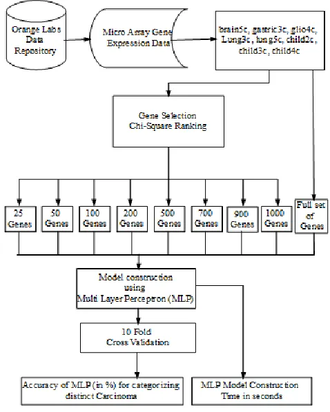
Lung cancer dataset with five diagnostic classes was collected and model was constructed using MLP. Figure 6 shows the performance obtained for lung5c dataset with optimal number of genes. It was identified that with full gene set, MLP gave an accuracy of 77% whereas after gene selection, MLP gave higher accuracy of 91% for top ranked 200 genes. Model construction time while using full gene set (12600) was 348 seconds which was decreased to 7.08 seconds for 1000 genes and it took only 1.38 seconds for top ranked 200 genes.

Fig 6. Performance of MLP in classifying lung cancer with five diagnostic classes

F. Childhood Leukemia with 2 Diagnostic classes

shows the performance obtained for child2c dataset with optimal number of genes. It was identified that with full gene set, MLP gave an accuracy of 57% whereas after gene selection, MLP gave higher accuracy of 100% for top ranked 1000 to 25 genes. Model construction time while using full gene set (9945) was 19.3 seconds which was decreased to 0.83 seconds for 1000 genes and it took only 0.02 seconds for top ranked 25 genes.

Fig 7. Performance of MLP in classifying childhood leukemia with two diagnostic classes

G. Childhood Leukemia with 3 Diagnostic classes

Childhood leukemia with three diagnostic classes was collected and model was constructed using MLP. Figure 8 shows the performance obtained for child3c dataset with optimal number of genes. It was identified that with full gene set, MLP gave an accuracy of 52% whereas after gene selection, MLP gave higher accuracy of 96% for top ranked 50 genes. Model construction time while using full gene set

(9945) was 18.3 seconds which was decreased to 0.73 seconds for 1000 genes and it took only 0.04 seconds for top ranked 50 genes.

Fig 8. Performance of MLP in classifying childhood leukemia with three diagnostic classes

H. Childhood Leukemia with 4 Diagnostic classes

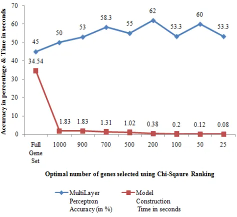
Childhood leukemia with four diagnostic classes was collected and model was constructed using MLP. Figure 9 shows the performance obtained for child4c dataset with optimal number of genes. It was identified that with full gene set, MLP gave an accuracy of 45% whereas after gene selection, MLP gave higher accuracy of 62% for top ranked 200 genes. Model construction time while using full gene set (8280) was 34.5 seconds which was decreased to 1.83 seconds for 1000 genes and it took only 0.38 seconds for top ranked 200 genes.

Table 1 depicts the performance of Chi-Square gene selection with MLP for full gene set and optimal gene set of each cancer type.

TABLEI.PERFORMANCE OF MLP FOR CATEGORIZING DISTINCT CARCINOMA

MGE Dataset

No. of Samples

Full Gene Set

Accuracy of Multi-Layer Perceptron (Full Gene Set)

Model Construction Time in seconds

(Full Gene Set)

Optimal Gene Set Chi-Square

Accuracy of Multi-Layer

Perceptron (Optimal Gene Set)

Model Construction Time in seconds (Optimal Gene Set)

brain5c 40 7129 45 17.5 50 82.5 _0.09

gastric3c 30 4522 73 6.32 25 80 _0.04

glio4c 50 12625 42 68.9 100 86 _0.18

lung3c 34 10541 59 33.7 700 91 _0.74

lung5c 203 12600 77 348 200 91 _1.38

child2c 23 9945 57 19.3 25 100 _0.02

child3c 23 9945 52 18.3 50 96 _0.04

Fig 9. Performance of MLP in classifying childhood leukemia with four diagnostic classes

VI. CONCLUSION

Microarray Gene Expression data has many genes compared to number of samples. MGE data is subject to noisy and irrelevant features which may lead to overfitting and impact the accuracy of a classifier. Thus gene selection has to be done prior to classifying any type of disease from gene data. Chi-Square gene selection method computes the correlation of one gene with the other and selects only top ranked genes. Multi-Layer Perceptron is a neural network algorithm which learns (constructs) the model in multiple iterations until the classification error rate becomes very minimal. MLP was widely used in gene expression data which motivated the authors to categorize eight different cancer types. From the results, it was identified that classification with full gene set yields very less accuracy, whereas gene selection followed by classification improves accuracy and also reduces model construction time. In future the work has to be extended by applying different activation functions in MLP and analyze the results. Further the authors were inspired by parallelized MLP and compare single run MLP with parallel run MLP.

REFERENCES

[1] Luque-Baena, Rafael Marcos, Daniel Urda, Jose Luis Subirats, Leonardo Franco, and Jose M. Jerez, “Application of genetic algorithms and constructive neural networks for the analysis of microarray cancer data.” Theoretical Biology and Medical

Modelling 11, no. 1, pp. 1-18, 2014.

[2] Bernardo, J. M., M. J. Bayarri, J. O. Berger, A. P. Dawid, D. Heckerman, A. F. M. Smith, and M. West, “Bayesian factor regression models in the “large p, small n” paradigm.” Bayesian statistics 7, pp. 733-742, 2003.

[3] Ransohoff, David F, “Rules of evidence for cancer molecular-marker discovery and validation.” Nature Reviews Cancer 4, no. 4, pp. 309- 314, 2004.

[4] Belciug, Smaranda, “A two stage decision model for breast cancer detection.” Annals of the University of Craiova-Mathematics and Computer Science Series 37, no. 2, pp. 27-37, 2010

[5] Saeys, Yvan, Iñaki Inza, and Pedro Larrañaga, “A review of feature selection techniques in bioinformatics.” bioinformatics 23, no. 19, pp. 2507-2517, 2007.

[6] Singhi, Surendra K., and Huan Liu, “Feature subset selection bias for classification learning.” In Proceedings of the 23rd international conference on Machine learning, pp. 849-856. ACM, 2006. [7] Hall, Mark A, “Correlation-based feature selection for machine

learning.” PhD Thesis, The University of Waikato, 1999.

[8] Tsang, Eric CC, Degang Chen, Daniel S. Yeung, Xi-Zhao Wang, and John WT Lee, “Attributes reduction using fuzzy rough sets.” IEEE Transactions on Fuzzy systems 16, no. 5, pp. 1130-1141, 2008. [9] Geng, Xiubo, Tie-Yan Liu, Tao Qin, and Hang Li, “Feature selection

for ranking.” In Proceedings of the 30th annual international ACM SIGIR conference on Research and development in information retrieval, pp. 407-414. ACM, 2007.

[10] Das, Sanmay, “Filters, wrappers and a boosting-based hybrid for feature selection” Proceedings of the Eighteenth International Conference on Machine Learning, pp. 74-81, 2001.

[11] gracia Jacob, Shomona, “Discovery of novel Oncogenic patterns using hybrid feature selection And rule mining.” Ph. D Thesis, Anna University, 2015.

[12] Han, J. and Micheline Kamber, “Data mining Concepts and Techniques”. Elsevier Second Edition, 2006.

[13] Raad, Ali, Ali Kalakech, and Mohammad Ayache, “Breast cancer classification using neural network approach: MLP and RBF.” Networks 7, vol. no. 8: 9, pp. 15 -19, 2012.

[14] Azad, Venu, “Comparing The Performance Of MLP With One Hidden Layer And MLP With Two Hidden Layers On

Mammography Mass Dataset.” architecture 13: 15. International Journal of Emerging Trends & Technology in Computer Science (IJETTCS), Vol 5: 1, pp. 54- 58, 2016.

[15] Berrar, Daniel P., C. Stephen Downes, and Werner Dubitzky, “Multiclass cancer classification using gene expression profiling and probabilistic neural networks.” In Proceedings of the Pacific Symposium on Biocomputing, vol. 8, pp. 5-16. 2003. [16] Mitchell T.M., Machine Learning. McGraw-Hill Book Co.,

Singapore, pp. 174-175, 1997.

[17] Subirats, José L., Leonardo Franco, and José M. Jerez, “C-Mantec: A novel constructive neural network algorithm incorporating

competition between neurons.” Neural Networks 26, pp. 130-140, 2012.

[18] Artificial Intelligence Orange Labs. Ljubljana, available at http://www.biolab.si/supp/bi-cancer/projections/

[19] Alonso-González, Carlos J., Q. Isaac Moro-Sancho, Arancha Simon- Hurtado, and Ricardo Varela-Arrabal, “Microarray gene expression classification with few genes: Criteria to combine attribute selection and classification methods.” Expert Systems with Applications 39, no. 8, pp. 7270-7280, 2012.