Czech Technical University in Prague Faculty of Electrical Engineering MASTER S THESIS. Karel Lenc

(1)

Czech Technical University in Prague

Faculty of Electrical Engineering

MASTER’S THESIS

Karel Lenc

Evaluation and Improvements of Image Interest Regions

Detectors and Descriptors

Thesis supervisor: Prof. Ing. Jiˇr´ı Matas, Ph.D

(2)

(3)

(4)

(5)

Prohl´

aˇ

sen´ı

Prohlaˇsuji, ˇze jsem pˇredloˇzenou práci vypracoval samostatnˇe a ˇze jsem uvedl veˇskeré pouˇzité informaˇcn´ı zdroje v souladu s Metodickým pokynem o dodrˇzován´ı etických princip˚u pˇri pˇr´ıpravˇe vysokoˇskolských závˇereˇcných prac´ı.

V Praze dne. . . . podpis

(6)

(7)

Acknowledgements

Hereby I would like to thank my supervisor Jiˇr´ı Matas for his leading and advices. Further, I would like to mention my colleagues from Centre of Machine Perception, mainly Michal Perˇdoch and Jan ˇSochman, who helped me greatly with numerous advices.

Thanks to Andrea Vedaldi for leading me during my stay in Visual Geometry Group at University of Oxford and that he allowed me to have this valuable experience. I would like to thank also to Relja Arandjelovi´c from VGG for his help with the Retrieval Benchmark design. My thanks also belong to my family and friends for their support, without which I would not be able to finish this work.

I acknowledge the financial support of PASCAL Harvest programme without which I would not be able to stay in Visual Geometry Group in University of Oxford participating to VL-Benchmarks project.

(8)

(9)

Abstract

A reliable and informative performance evaluation of local feature detectors and descriptors is a difficult task that needs to take into account many applications and desired properties of the local features. The main contribution of this work is the extension of the VLBenchmarks project which intends to collect major evaluation protocols of local feature detectors and descriptors.

We propose a new benchmark which evaluates local feature detectors in the image retrieval tasks and simple epipolar criterion for testing detectors and descriptors in the wide baseline stereo problems. Using the extended benchmarks we investigate several parameters of the local feature detection algorithms.

We propose a new algorithm for building a scale space pyramid which significantly im-proves the detector repeatability in the case of apriori knowledge of the nominal Gaussian blur in the input image. On the image retrieval tasks, we show that features with a small value of the response function improve the performance more than features with small scale, contrary to the observations in the geometry precision benchmarks. By altering the compu-tation of the SIFT descriptor, we show that it is not necessary to weight the patch gradient magnitudes when input images are similarly oriented and that for blob-like features increasing the measurement region improves the performance.

Finally we propose an improvement of emulated detectors that allows finding new image features with better geometric precision. We have also improved the classification time of the emulated detectors and achieved higher performance than the handcrafted OpenSURF detector implementation.

Abstrakt

Spolehlivé a dostateˇcnˇe informativn´ı mˇeˇren´ı výkonnosti detektor˚u zájmových oblast´ı nen´ı snadným úkolem a závis´ı jak na konkrétn´ı aplikaci, tak i na jejich poˇzadovaných vlastnostech. Hlavn´ım pˇr´ınosem této práce je rozˇs´ıˇren´ı open source projektu VLBenchmarks, který se snaˇz´ı nashromáˇzdit hlavn´ı protokoly pro mˇeˇren´ı vlastnost´ı detektor˚u zájmových oblast´ı a jejich deskriptor˚u.

V rámci práce jsme navrhli nový testovac´ı protokol mˇeˇr´ıc´ı výkonnost detektor˚u a deskrip-tor˚u zájmových oblast´ı pouˇzitelných v systémech pro vyhledáván´ı instanc´ı obraz˚u v rozsáhlých databáz´ıch. Dále jsme navrhli jednoduché kritérium pro testován´ı detektor˚u a deskriptor˚u ve wide-baseline dvou-pohledových geometri´ıch. S pomoc´ı tˇechto nových testovac´ıch protokol˚u jsme prozkoumali nˇekolik nejd˚uleˇzitˇejˇs´ıch parametr˚u algoritm˚u pro detekci zájmových oblast´ı. Navrhli jsme nový algoritmus pro stavbu pyramid prostoru mˇeˇr´ıtek, jenˇz zvyˇsuje opako-vatelnost detektor˚u v pˇr´ıpadˇe znalosti Gaussovského jádra, kterým byl obrázek rozmazán. Na systému pro vyhledáván´ı obraz˚u jsme ukázali, ˇze pˇri zahrnut´ı zájmových oblast´ı s niˇzˇs´ım kontrastem, lze významnˇeji zvýˇsit jejich pˇresnost, neˇz pˇri zahrnut´ı oblast´ı s menˇs´ı velikost´ı. Ukazujeme ale, ˇze toto neplat´ı pro pˇr´ıpady pouˇzit´ı, kde je upˇrednostˇnovaná geometrická pˇresnost detekce. Na pˇr´ıpadˇe ˇsiroce pouˇz´ıvaného SIFT deskriptoru ukazujeme, ˇze pokud data, na nichˇz je poˇc´ıtán, neobsahuj´ı významné rotace, nen´ı potˇreba vstupn´ı data deskrip-toru váˇzit Gaussovským jádrem. S tˇemito protokoly jsme také zmˇeˇrili výkonnost detektor˚u a deskriptor˚u z hlediska velikosti oblasti, která je pouˇzita pro výpoˇcet deskriptoru. Ukazuje se, ˇze pro detektory isotropn´ıch oblast´ı se vˇzdy dosáhne lepˇs´ıch výsledk˚u, pokud je do výpoˇctu deskriptoru zahrnuto v´ıce kontextu detekované oblasti.

V posledn´ı ˇcásti této práce navrhujeme vylepˇsen´ı emulátor˚u detektor˚u zájmových oblast´ı, které dovoluje detekovat nové typy zájmových oblast´ı a zvyˇsuje jejich geometrickou pˇresnost. Také jsme významnˇe zvýˇsili efektivnost tˇechto emulátor˚u tak, ˇze dosahuj´ı vyˇsˇs´ı rychlosti detekce, neˇz z hlediska rychlosti peˇclivˇe navrˇzený OpenSURF detektor.

(10)

(11)

Chapter

1

Introduction

In the field of computer vision, local image feature detection is an intermediate step of several algorithms. It is used for representing an image by a set of well defined and well localised image structures with an informative neighbourhood. Typically some set of measurements are taken from the feature neighbourhood to form a descriptor. Image features and their descriptors are used in many applications e.g. in multiple view geometry (e.g. image stitching, structure from motion and 3D reconstruction), object recognition and image retrieval.

A local image feature is an image pattern which differs from its immediate neighbourhood. They are interesting because they can provide a limited set of well localised and individually identifiable anchor points. What they represent is not relevant so far as their location can be determined accurately and in a stable manner over time. In multiple view geometry what is important is their location (centre) as they are used for estimation of the scene model. In other cases the set of local features and their descriptors can be used as a robust image representation that allows to recognise objects and scenes without a need for segmentation. In this case they do not have to be localised precisely since to analyse their statistics is more important [41].

A detector is a tool that extracts features from an image (usually corners, blobs etc.). An ideal extracted feature should have several properties such as repeatability, distinctiveness (informativeness) and precise localisation. However, these properties change with the detec-tor parameters not only depending on the type of features which it extracts, but also on a particular implementation. This puts us in a difficult task how to properly measure these properties. Existing and widely used performance evaluation protocols are limited to test detectors only on planar scenes which does not address problems such as occlusion or depth discontinuities. Also it does not directly address the properties required for image retrieval where the feature localisation is not so important. This motivates our first goal which is to make it easier to test any feature detector or descriptor algorithm not only with existing tests but also with newly proposed benchmarks which would confront other use cases of these algorithms. With this evaluation framework we would like to examine performance of feature detectors and subsequently their descriptors in order to set their parameters depending on their particular use.

Next goal of this work is to examine emulated feature detectors proposed in [38]. These emulators offer a possibility to speed up several feature detector algorithms. In the original article [37] they had been tested only with benchmarks consisting of planar scenes experiments. Thus they are tested in the proposed new benchmarks in order to asses their performance in retrieval and epipolar geometry tasks. Subsequently we train emulators of different local image features and examine their properties.

(14)

1.1 Main contributions

One of the contribution is participation in VLBenchmarks framework which is an auxiliary suite of tests for VLFeat computer vision library algorithms. We have finalised implementation of existing evaluation protocols and proposed new evaluation protocols such as the Epipolar geometry test and image retrieval benchmark. These tests has been implemented under supervision of Andrea Vedaldi in Visual Geometry Group, University of Oxford during May and August 2012. The VLBenchmarks project was presented as a part of a tutorial at ECCV 2012 in Firenze. Using VLBenchmarks software we have tested several properties of existing detectors.

We propose a new algorithm to build a pyramid Gaussian scale space which allows to take into account any nominal Gaussian blur in a processed image. With a-priory knowledge of this blur it is able to increase repeatability of scale space local feature detectors significantly. A new method to control number of detected features has been proposed by setting lower initial scale. Employing VLBenchmarks tests we have found that for geometry precision tasks it is better to increase the number of detections by detecting smaller features with lower initial scale. However for retrieval tasks, features with lower response function threshold are more advantageous than features with small scale. We have shown, that for some retrieval tasks, where the scale of queried and database instances is similar, it is possible to decrease the number of features in the database as the smallest features has got little impact to retrieval system performance.

Last parameter examined is measurement region of a local feature used for descriptor calculation. We show that for blob detectors, bigger measurement region generally improves their performance mainly for planar scenes. This however does not hold for Harris and MSER detector where the ideal measurement scale is limited. Also we have shown that for input data without significant rotations descriptors are more distinctive without weighting.

In the last part we train new emulated detectors using different local image features than in the original article. We have shown that it is also possible to train detectors with anisotropic features however with the cost of worse rotation invariance. Using VLBenchmarks, newly trained DoG emulated detector gains better geometric precision than the original Hessian-Laplace emulator. Besides that we have improved the classification speed so that the emulators achieve faster evaluation than SURF detector.

1.2 Structure of this thesis

In Chapter 2 we describe existing feature detection algorithms and their emulators. In the next part, Chapter 3, existing evaluation protocols for feature detectors and descriptors are described. Then we follow with description of our work on VLBenchmarks project in Chapter 4. Using this evaluation framework we examine detectors parameters in Chapter 5. In Chapter 6 we follow with description of improvements and tests performed with emulated detectors. In the last part, Chapter 7, we summarise the results.

(15)

Chapter

2

Local image features detection and

description

In this chapter we describe state of the art algorithms for local feature detection and descrip-tion. Local image features can be divided based on the invariance to image transformations or by the feature type. The major types of local features areblobs (LoG, DoG and Hessian),

corners (Harris) and regions (MSER). In the first section, we describe classes of invariance to geometric transformations. Then we follow with a detailed description of feature detectors which use scale space extrema of second order derivative operators as a tool to obtain both feature location and scale. Then other feature detectors and main algorithms for feature de-scription are briefly described. The local image feature detection can also be seen as a decision process, we will show that it is possible to use machine learning techniques to emulate it. The underlying theory for boosting and emulated detectors is described in the last part of this chapter.

Notes on terminology In the text we use several terms for a local image feature. This

ambiguity arises from their different use. For some applications (3D reconstruction or camera calibration) the spatial extent of the local image feature is not important and only the feature location is used. The term interest pointis then often used. In most applications, where the regions has to be described, such that they can be identified and matched, one typically uses termregion instead of interest point [41, p. 182]. In this work we use the termlocal feature

or termframe, which will be described below.

2.1 Local image features and their invariance

Local image features are deterministic local image statistics (features) robust to several types of image distortion factors such as viewpoint change or change of illumination [42], and which differ from their immediate neighbourhood. By definition they are well localised to a compact subset of an image which will be further referred as a region of the feature. The desired property of the feature is an invariance to a particular parameter or function applied to the original image domain.

Local features are detected withcovariant local image feature detectors (detectors) which select a number of distinctive image regions from the input image. The detector is covariant with a particular family of transformations when the shape of detected image regions does change with the image transformation [41, p. 181]. One way to obtain invariance of the local features comes from the geometric, photometric normalisation [41] of the detected image regions. The idea is that once the local image regions that were found under the image distortion are normalised into a canonical shape, any measurement on the normalised regions are invariant to the deformation. The image regions obtained by the local feature detectors

(16)

(x0, σ)

Disc Oriented Disc Ellipse Oriented Ellipse

(x0, σ, θ) (x0,Σ) (x0, A)

σ

σ θ

z

x0 x0 x0 x0

Figure 2.1: Classes of the local image frames.

Frame class Attributes Covariant to

Disc Frame coordinates x0, scale (radius)σ Translations and scaling

Oriented Disc Frame coordinates x0, scale (radius)σ Translations, scaling

and single pointzwhich defines orientationθ and rotation (similarities)

Ellipse Frame coordinates x0and shape matrix Σ Translation and affinities

with three degrees of freedom up to residual rotations

Oriented Ellipse Frame coordinates x0 Translation and affinities.

and affine transformationA

Table 2.1: Attributes of image frame invariance classes.

are represented by geometric entities denoted as frames. A frame is a subset of the image, defined by a set of attributes that uniquely specifies particular geometric shape, for example disc or ellipse. A class of frames are frames that can be specified by the same set of attributes. The overview of frequently used classes of local image feature frames is given in table 2.1 and visualised together with their attributes in Figure 2.1. This categorisation and description of the frames is based on [42]. Let us now describe the properties of these frame classes:

Disc Compact subset of the image, Ω =_{|x₋x0|< r}, represents a circular region in the

image.

Oriented disc Set Ω (defined as above) and a pointzwhich defines the major orientation

of the circular region. This major orientation can be also expressed by an angle θ, which is the angle of the the linex0×z.

Ellipse Frames defined by their centre x0 and the moment of inertia (covariance) matrix

(also further referred as second moment matrix). Σ =R 1

Ω1dx

Z

Ω

(x₋x0)(x−x0)Tdx (2.1)

The covariance matrix is positive semi-definite 2_×2 matrix that can be visualised by an ellipse [13] as:

(x₋x0)T Σ−1 (x−x0) = 1 (2.2)

Ellipse behaves similarly as a covariance matrix of image region under the affine transforma-tions and is useful for intuitive prediction of the feature frame behaviour. This also is a reason why we further refer to the covariance matrix as an ellipse matrix. For details and a proof see [13, p. 5].

Oriented ellipse Oriented ellipses are defined by an affine transformationA which

trans-forms an oriented ellipse ΩC into an oriented unit disc AΩ = ΩC with orientation θ = 0

(17)

The local feature detector is an algorithm that finds a mappingF_{from image domain}_I(_x₎ to attributed frames domain Φ, where the the detections are uniquely described by the values of frame attributes.

2.2 Detection of local image features with scale space

The scale space based feature detectors search for a local feature inspatialandscaledomains of an image using some “distinctiveness” measurement (either a cornerness or a blob measure, further noted as aresponse function). This is generally a search in a three dimensional space, where the third dimension can be seen as a sampling of spatial frequency domain. The feature detection can be divided into three steps:

1. The scale space extrema localisation Search of local extrema in the scale space of the

image response function.

2. Location refinement Sub-pixel localisation of the frame centroid and scale based on a

local optimisation.

3. Additional measurements that improves covariance of the detector. The image regions

obtained as local extrema in the scale space are uniquely determined by a disc frame attributes (x,y, σ). The disc frame can be “upgraded” by further examination of the image region to an oriented disc, ellipse or oriented ellipse. The ellipse frame can be estimated by using Baumberg iteration [4]. The oriented frames can be obtained by computing the dominant orientation of the image gradients in the normalized coordinate frame [24].

2.2.1 Gaussian scale space properties

The Gaussian scale space is a multi-scale representation of the original image computed by consecutive filtering of the input image. The consecutive application of a low pass Gaussian filter allows to analyse lower resolutions of the image. The choice of the Gaussian filter among the low pass filters is not random, it has been shown [21] that the Gaussian scale space is a natural solution to a diffusion equation. The Gaussian scale space also holds several important properties, asshift invariance,scale invariance,rotational symmetry and mainlynon-creation of local extrema or zero-crossings in the one-dimensional case(non-enhancement property)[23, p. 3].

The Gaussian scale space is a continuous functionL(x, σ) of some input imageI(x) defined as:

L(x, σ) =G(x, σ)_∗I(x) (2.3)

where ∗denotes a convolution of the input image and the Gaussian kernel: G(x, σ) = 1

2πσ2e

−xTx/2σ2

(2.4) The local feature detectors based on the Gaussian scale space use properties of second order derivative operators. The amplitude of spatial derivatives

Lxi_yj(·, σ) =∂_xi_yjL(·, σ) =G_xi_yj(·, σ)∗I(·) (2.5) generallydecrease with scaledue to non-enhancing of local extrema property of the Gaussian kernel. In order to be able to compare the derivatives across scales, the derivative operator responses across the scales, the amplitude of Gaussian derivatives must be normalised by a factor [22]:

ˆ

Lxi_yj(·, σ) =σ(i+j)γL(·, σ) (2.6) Where in the most cases ([24], [27]) the parameterγ is selected asγ= 1.

(18)

2.2.2 The scale space implementation

The scale space is by definition a continuous function, however the input image is not of infinite resolution. Therefore, a discrete approximation has to be made. The input image is assumed to be pre-smoothed in the discretisation process by a Gaussian low pass filter with some nominal standard deviation σn= 0.5. Due to computation efficiency, the scale space is

sampled into a finite number of scales by cascade convolution of the image using the Gaussian kernel. This is possible thanks to the following property of the Gaussian kernel:

G(x, σ2)∗G(x, σ1)∗I(x, y) =G x,qσ2 1+σ22 ∗I(x, y) (2.7)

This means that for computation of each successive layer of the scale space we can reuse the previous layer. The scale space construction is made even faster by constructing a pyramid where the scale space is divided into octaves v such that each following octave doubles the scale of previous one. Scales are then sampled exponentially, such that after each octave, the scale doubles:

σ=σ0 2v+

s

S s= 0, ..., S−1 v= 0, ..., v_max (2.8) Parameter σ0 = 1.6 is a scale of a pyramid base and was empirically set in [24, p. 10]

and represents the sampling frequency in the image domain (“given that extrema can be arbitrary close together, there will be a similar trade-off between sampling frequency and rate of detection” [24, p. 10]). The maximum number of octavesvmax is set to a value where the

longer size of the image is still bigger than 23_{. Each octave is down-sampled by factor 2.}

2.2.3 Local image feature localisation

Local features are detected as local extrema of some response function Resp(x, σD). The

size of the searched local neighbourhood is usually 3_×3_×3. The definition of the response function differs for each detector. The most widely used are:

Determinant of Hessian. For detecting distinctive features, the determinant of

Hes-sian [29] matrix measure is used. The HesHes-sian matrix is defined as: H(x, σD) = Lxx(x, σD) Lxy(x, σD) Lxy(x, σD) Lyy(x, σD) , (2.9)

where valuesLab(x, σD) are second order Gaussian derivatives of scale space valuesL(x, σD) (

σDis differential scale, also called local scale). The measure itself is defined as a determinant

of the Hessian matrix:

RespHess(x, σD) =σD2|H(x, σD)|, (2.10)

factor σ2

D is the normalisation factor of the second derivatives, in order to maintain scale

invariance of the response function across the scale levels. The determinant of Hessian re-sponse can be computed efficiently by computing symmetric differences in a 3_×3 window around each pixel. The response function has three types of extrema which correspond to the following types of Hessian features:

a) Bright blobwhen _|H(x, σD)|>0 andLxx<0. This feature correspond to “hill top”

blobs in image brightness.

b) Dark blob when |H(x, σD)| > 0 and Lxx > 0. This feature correspond to “valley”

blobs in image brightness.

(19)

Laplacian of Gaussian (LoG). The Laplacian of Gaussian response for blob detection is defined as the trace of the Hessian matrix:

RespLoG(x, σD) =σDtrace(H(x, σD)) (2.11)

And the features can be of type:

a) Bright blobwhen RespLoG(x, σD)<0

b) Dark blobwhen RespLoG(x, σD)>0

Difference of Gaussian (DoG). The difference of Gaussian [24] is an approximation

of Laplacian of Gaussian. The advantage of this response is that, in the scale space, it is computed without the convolution simply by subtracting the successive levels of scale-space:

RespDoG(x, σD) =

σD

∆ (L(x, σD+ ∆)−L(x, σD−∆)) (2.12) Feature types are categorised in the same way as for the LoG response.

Scale adapted Harris response (Harris). The response function of the Harris corner

detector [27] is based on the second moment matrix of image gradients, also called an auto-correlation matrix. It is defined as:

M(x, σD, σI) =σ2DG(x, σD)∗ L2 x(x, σD) Lx(x, σD)Ly(x, σD) Lx(x, σD)Ly(x, σD) L2y(x, σD) (2.13) where Lx are first order Gaussian derivatives with derivation scale σD. The outer products

of the gradients are averaged in the point neighbourhood with a Gaussian window of scaleσI

(integration scale). The eigenvalues of this matrix represent the principal changes of image intensities in two orthogonal directions. Their ratio is effectively computed with the Harris corner measure:

RespHarr(x, σD) =|M(x, σD, σI)| −λtrace(M(x, σD, σI)), (2.14)

with typically λ= 0.04 and σI =√2 σD (in case of CMP implementation). Only response

function maxima are considered by the detector.

For scale estimation, the Laplace operator is usually used in a hybrid detector. Hybrid detectors are described below.

Sub-pixel/Sub-scale localisation

At higher levels in the scale space pyramid, it is important to localise the feature more precisely as there the pixels correspond to large areas relative to the base image [6]. It is supposed that the response function is smooth enough around the extrema that it can be approximated with a 3D quadratic function. The 3D quadratic function is then fitted into a 3_×3_×3 neighbourhood of the local extrema and its peak is taken as a sub-pixel and sub-scale location [6]. The function is expressed in a Taylor expansion (up to quadratic elements) of the scale space function Resp(x, σ) with the origin in a location of the scale space extremum.

Resp(z) = Resp +∂Resp ∂z T z+1 2z T∂2Resp ∂z2 z (2.15)

Where vectorz= (x′, σ′)T _{is the offset from the localised point. The location of the extremum}

of this function ˆz, i.e. our solution offset can be obtained as: ˆ z= ∂ 2_Resp ∂z2 −1 ∂Resp ∂z (2.16)

This is an easily solvable 3_×3 linear system. If the offset is bigger than ˆz>0.6, it means that the extremum lies closer to a neighbouring point, so the detected location is changed and the optimisation is run again in an iterative procedure (in our case limited to maximum of five steps) until the location is found stable. The final offset ˆzis added to the feature location.

(20)

2.2.4 Low contrast and edge regions suppression

The second order derivatives based detectors fire on the edges, where at least one of the second derivatives is high. To eliminate the edge responses which tend to be unstable under geometric transformations1, the Hessian matrixH of the response function is used. Its eigen-values (λmax, λmin) are proportional to the principal curvatures of the response function.

Because only the ratio between the eigen-values r = λmax/λmin is important, it can be

calculated as comparison of the trace and determinant of the Hessian matrix: Tr(H)2 Det(H) = (λmax+λmin)2 λmaxλmin = (r+ 1) 2 r (2.17)

and only regions which fulfil the following condition Tr(H)2

Det(H) <

(r+ 1)2

r (2.18)

are preserved [24].

Also in order to suppress regions with low contrast, only regions with response higher than aresponse function threshold Rt(also called peak threshold) are preserved.

2.2.5 Estimation of feature orientation

The local features detected in the scale space are assigned with a location and scale, and represented by a disc frame that does not provide information about feature orientation. However, the feature can be upgraded to an oriented disc to increase the invariance of the descriptors computed on the detection. One of the ways how to find a robust orientation of the feature is to exploit local gradients in the vicinity of the feature.

The gradient orientationsθ(x) and magnitudesm(x) in a circular region with radiusrwin=

1.5σ are computed (VLFeat SIFT2_{) at the closest scale level of the pyramid corresponding}

to the detected scale of the feature. Then, the gradient orientation are weighted by gradient magnitudes and collected in an orientation histogram additionally weighted by the gradient magnitudes. Gradient magnitudes are weighted by a Gaussian kernel with σ = 1/3 rwin

in order to emphasise gradients closer to local feature’s centre. The number of bins of the histogram is usually set to 36.

After smoothing the histogram values, in order to remove coarse peaks, local peaks within 80% of the global maxima are returned as the detected orientations. The maximum number of extrema is usually limited to 4. In case the full affine invariance (oriented ellipse) is desired, the orientation is computed on patch normalised to a unit disc, to allow affine covariant measurements of the gradient orientations.

2.2.6 Hybrid detectors

We denote scale-space based detectors as hybrid, when the response function in the spatial domain differs from the response function used to find the scale of the feature. The hybrid detectors proceeds as folloe. First, a spatial local feature location is found using a non-maxima-suppression in the 3_×3 neighbourhood on each scale level independently. Then, the best scale is found an extremum of the second measure over all scales. Common combinations of response functions used in the literature are Harris-Laplace [27] orHessian-Laplace [29] mainly for the good localisation of the corner-like features by the Harris response function.

2.2.7 Affine invariance

Baumberg [4] has shown, that a disc frame can be extended to an ellipse frame by an algorithm called Baumberg iteration. This algorithm iteratively estimates the affine distortion of the

1

Location on the edge is well defined only in the direction orthogonal to the edge. 2

(21)

gradients of the detected feature by computing a structure tensor with the second moment matrix of image gradients, which is used as a measure of anisotropy. In each step, the inverse square root of the second moment matrix is accumulated and the accumulated transformation used as an estimate of affine distortion. The estimated affine transformation is then used to normalise an image patch around the feature. The iteration continues, until sufficient isotropy of the normalised patch is achieved. This iteration removes frames where the iteration does not converge. This usually happens for too elongated features (such as edges). The result of the iteration is an affine transformation that is fixed up to an unknown rotation3_{. This}

rotation can be fixed as upright [31] (ellipse frame), or dominant orientation can be estimated as described above to form an oriented ellipse. Detectors which use Baumberg iteration are further referred with the -Affinesuffix.

2.3 Other state of the art detectors

Besides the already introduced scale space detectors plentiful of other feature detectors exist. We present a small selection of the most important ones.

MSER [26] Region detector based on a modified watershed algorithm with different sta-bility criteria. In general it detects regions, however they are usually converted to ellipses where the centre is defined as their centre of gravity and the shape is specified by moments of the detected region interior. The scale of the ellipse is then usually twice the scale defined by the moments. Generally it detects fewer regions but the detected features are naturally affine invariant.

SURF [5] Speed Up Robust Features. The similarity invariant frame detector, which comes with the SURF descriptor, detects frames using an approximation of the Hessian response with box filters. The orientation of the frames is fixed using box filters. In some sense, it is similar to emulated detectors, as the box filters resemble Haar features computed with assistance of integral images. However, the particular filters are carefully engineered and their response is used directly. The scale of the features is detected over a pyramid of box filter size which partly resembles the scale space pyramid and it uses the same non-maxima suppression as the scale space detectors, together with sub-pixel localisation.

FAST [34] A translation and rotation invariant corner detector (no scale invariance) which uses a decision tree to classify a possible feature presence by comparing central pixel to its 12 pixel circular neighbourhood (in this sense it is somehow similar to local binary patterns). The decision tree is learnt using machine learning techniques to achieve decision in the shortest time. In comparison to other detectors, FAST simplicity bringsfastdetection though without scale invariance.

BRISK [20] The detector used in this framework is an extension of the FAST detector

with a Gaussian scale space. A classical non-maxima suppression over the FAST score is performed in order to locate the features in the scale dimension. Sub-pixel localisation is also performed.

2.4 Local image feature description

The local feature descriptors provide a description invariant to the image transformation. This can be achieved mainly by two means: either by descriptors invariant to the transfor-mation e.g. rotation, or by descriptors that are not invariant to the transfortransfor-mation, however computed on the neighbourhood normalised using the detected covariant frame. This two approaches can be also combined. The geometric normalization proceeds as follows. At first,

3

(22)

the detection scale is multiplied by a magnification factor ν in order to obtain more distinc-tive neighbourhood a feature’smeasurement region. The measurement region of the feature is then normalised (usually rotation or affine shape normalisation) to a small patchP (usually of size 41 pixels) which is then used for calculation of an invariant descriptor.

Descriptors are robust image transformations which characterise the image brightness structures and are invariant to photometric transformations. Let us introduce some of the commonly used local feature descriptors:

SIFT [24] The SIFT descriptor is a 3D spatial histogram capturing the spatial distribution, magnitude and orientation of the image gradients [43]. The image gradients are collected in a 4_×4 grid (to preserve spatial information) where each cell is described by a histogram of image gradient orientations inside the cell. Each histogram is expressed by eight values yielding a 4_×4_×8 = 128 values long descriptor. Thanks to this coarse spatial division, this descriptor is robust to some errors in local feature position and orientation. Collected values are then quantized to fit into one byte. The similarity measure is the Euclidean distance or Hellinger distance (RootSIFT, [3]).

SURF [5] SURF descriptor is calculated with box filter similarly as the SURF features. The spatial and orientation information is stored in a similar way as in SIFT. However the descriptor is only 64 bytes long. The similarity measure used is usually the Euclidean distance.

BRIEF [7] (Binary Robust Independent Elementary Features). A binary vector which

consists of results of a certain number of pairwise (or n-wise) intensity comparisons in a smoothed patch. The patch is sampled randomly with a bias towards the patch centre. The advantage of binary descriptors is their small memory footprint as results of each comparison are stored in a single bit. Similarity is computed with Hamming distance, which can be quickly performed with an XOR operator and a processor instruction which counts the number of zero bits.

DAISY [40] This descriptor collects its values by sampling orientation maps (gradients

of the patch in particular directions) by averaging values in a small neighbourhood with a Gaussian kernel. Samples are taken on a circular pattern where the size of the averaged neighbourhood increases with the circle radius. This creates a Daisy-like structure. This de-scriptor was developed mainly for dense stereo matching. In [48], machine learning techniques are used for learning to pick the best samples with a goal to form a compact and distinctive descriptor.

LIOP [47] Instead of gradients, LIOP collects histograms of pixel orderings. First, it divides image brightness values into several bins. In each bin, N pixel samples are taken on a circular pattern around the centre of the feature and pixel intensities ordering are collected into a histogram of N! bins. Concatenated ordering histograms over all bins form the LIOP descriptor. The similarity measure used is Euclidean distance, however as it is formed by histograms, Hellinger distance may be used as well.

MROGH [10] Extension of LIOP descriptors where several LIOPs over different

(23)

· · · =_⇒

Figure 2.2: The multi-scale sliding window approach to detection. A detection window is swept through the image and an object vs. background classifier is evaluated at each position and scale.

2.5 Emulated local feature detectors

The concept of emulated local image feature detectors has been introduced in [38]. It is based on WaldBoost learning framework [37], applied to detection of the local image features. The task is to learn a sequential classifier which is able to decide whether a given image sample contains an image feature or not.

The key idea is, that some existing feature detection algorithm is used as a black box algorithm performing a binary decision task. Running this algorithm on a big set of images it provides a large amount of positive and negative samples for training of the classifier. Then the classifier is used to emulate the black box algorithm of the feature detector. It detects features in the image by classifying all rectangular regions (patches) of various sizes and in various positions, by using a multi-scale sliding window technique. The sliding window approach is illustrated in Figure 2.2.

Considering the size of the image and the number of possible scales, the sliding window technique produces ample amount of patches which need to be classified. This task was first solved in real time by Viola and Jones [44]. Based on the extensive research in the field of real-time image detectors the emulated feature detectors use a Waldboost algorithm [37] to emulate the Hessian-Laplace [27] and Kadir-Brady saliency detector [16]. The main advantage of the emulated detectors is their speed, as the WaldBoost sequential classifier is able to eliminate an ample amount of background patches by early decision.

In the following, we describe some basics about the WaldBoost sequential classifier and RealBoost used for selection of the weak classifiers. Then, we continue with details related to emulated local image feature detectors.

2.5.1 WaldBoost

WaldBoost is a meta algorithm, an extension of AdaBoost meta-algorithm [12], which allows to make an early decision and therefore speed-up the classification. But instead of using a cascade of separate strong classifiers as Viola and Jones [44], the number of measurements needed is decided using a sequential probability ratio test.

Sequential probability ratio test Sequential probability ratio test(SPRT) is a statistical

framework developed for quality control in manufacturing proposed by Wald [46]. It is useful for decision making when the number of samples is not known in advance. By continuously collecting the data, the decision is postponed until sufficient information is available. The advantage of this approach is that the decision can be made much earlier than in the case of non-sequential, monotonic, algorithms.

Let x be an object with hidden state (class, label) y _{∈ {−}1,+1_} which is not directly observable. The hidden state is determined based on successive measurements x1, x2, . . .

and the knowledge of joint conditional probabilities p(x1, . . . , xt|y = c) of the sequence of

(24)

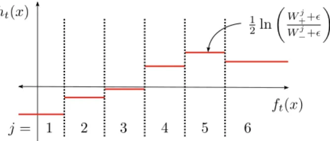
ht(x) ft(x) j = 1 2 3 4 5 6 1 2ln W+j+ǫ Wj −+ǫ

Figure 2.3: The domain-partitioning weak classifier, also known as RealBoost weak classifier. The response of features f(x) on a samplexis partitioned into bins j= 1, . . . , K. The left-most and right-left-most bins cover respective half-spaces. In each binj, the response of the weak classifierh(x) is learnt from the sum of positive (W+j) and negative (W−j) weights falling into

the bin. The sample weights are set according to AdaBoost learning strategy [12]. To avoid numerical problems, a smoothing factorǫis used [35]. Adopted from [38].

defined as [46]: St∗=      +1 ifRt≤B −1 ifRt≥A # ifB < Rm< A (2.19) The symbol # stands for “continue”, i.e. do not decide yet. Rtis defined as a likelihood

ratio:

Rt=

p(x1, . . . , xt|y=−1)

p(x1, . . . , xt|y= +1)

(2.20) And the constantsAandBare set accordingly depending on the required probability of error of first kindα(xbelongs to +1 but is classified as₋1) and probability of error of the second kindβ (xbelongs to₋1 but is classified as +1). It is generally difficult to estimate the values ofAandB. Wald [46] suggests to set them to their upper and lower bounds respectively:

A′=1−β

α , B

′₌ β

1₋α (2.21)

Following this decision, in [37] the t-dimensional space is projected into a one dimensional space by a boosted strong classifier functionHtof lengthtand the likelihood ratio is estimated

as: ˆ Rt= p(Ht(x)|y=−1) p(Ht(x)|y= +1) (2.22) Moreover, ˇSochman and Matas [37, p. 4] shows that this projection sufficiently approximates the ˆRt. The strong classifier of lengthT is defined as:

HT(x) = T

X

t=1

ht(x) (2.23)

Whereht(x) are responses of the weak classifiers.

Weak classifier selection The RealBoost domain partitioning weak classifiersht[35] are

used, each one based on a single (visual) featureft(see Figure 2.3).

The input to the WaldBoost learning algorithm is a pool of samples_P, a set of features_F and the bounds on the final false negative rateαand false positive weightβ. In the learning, the selection of the weak classifier is by far the most time consuming operation. Therefore only a subset_T of the samples pool _P is used for selection of the weak classifier. In each round, the already decidable samples in the pool are removed from the learning process and new training set T is sampled. This process is called Bootstrapping. Details about the learning with bootstrapping are shown in Algorithm 1.

(25)

Algorithm 1 WaldBoost learning with bootstrapping, adopted from [38]

Input: Sample poolP ={(x1, y1), . . . ,(xm, ym)};xi∈ X, yi∈ {−1,+1}, set of features F= {fs}maximal false negative rateαand false positive rateβ, number of weak classifiersT

1: Sample randomly the initial training setT from the poolP

2: SetA= (1−β)/αandB =β/(1−α) 3: fort= 1, . . . , T do

4: Choose best weak classifier ht by RealBoost [35] using F and T and add it to the

strong classifierHt. See Figure 2.3.

5: Estimate the likelihood ratio according to eq. 2.22 6: Find thresholdsθ_A(t)andθ_B(t)forHtbased onA,B

7: Bootstrap: Throw away samples from training set for which Ht ≥ θ_B(t) or Ht ≤ θ(_At)

and sample new samples into the training setT using QWS+ [18]

8: end for

returnstrong classifierHtand thresholdsθ(AT) andθ

(T) B . ... Th re sh ol d

Object Object Object

Background Background Background

Object

Background Image

0

don’t know don’t know

h1(x) h2(x) hT(x)

H1(x) HT−1(x) HT(x)

(26)

”Black Box” Vision Algorithm output binary images images Bootstrap management Image pool data request sample?

training Wald decision

Emulator Training Set _Learning WaldBoost ft, θ(At), θ (t) B samples labels

Figure 2.5: Learning scheme of feature emulator [38]. .

Sequential binary classifier The sequential binary classifier, as defined in [37], consists

of a set of weak classifiers as illustrated in Figure 2.4. A sequential classifier, denoted as St, sequentially computes responses of weak classifiers h1(x). . . ht(x) on input image patch

x. The responsesht(x) are summed up to the final response HT(x), the strong WaldBoost

classifier. The response HT(x) is then compared to the corresponding thresholds and it

is either classified positive or negative, or the next weak classifier is evaluated [38]. The difference from the traditional AdaBoost strong classifier is that in any step, based on the collected response, the final decision can be made. The sequential strategy is:

St(x) =      +1 ifHt(x)≥θB(t) −1 if Ht(x)≤θA(t) # if otherwise (2.24)

If a samplexis not classified even after evaluation of the last weak classifier, a user defined thresholdγis imposed on the real-valued responseHT(x) [38].

2.5.2 Feature detector emulators

In the scheme proposed in [38], the existing local feature detection algorithms are approached as black-box algorithms which perform a binary decision task. A scheme of the learning process is shown in Figure 2.5. Negative samples are any image patches which are not detected as local image features by the detector. For the emulators, the set_Fincludes Haar-like features proposed by Viola and Jones [44], plus a centre surround Haar-like features which has been shown to be useful in blob detection. An advantage of Haar features is that they can be efficiently evaluated using a integral image.

In the original articles, Hessian Laplace [27] and Kadir-Brady saliency [16] detectors are emulated. For learning, same Haar features as in [44] are used together with centre surrounded features which are useful for blob detection. Also, contrary to [37], feature responses are not normalised by the window standard deviation since the image brightness contrast is important for local image features. The classifier length is set toT = 20 as longer classifiers slow down the evaluation and do not bring significant improvement in the performance [38, p. 155]. In all experiments performed in [38],_{|T |}= 10,000, half positive and half negative samples.

Non maxima suppression An essential part of the detector is non-maxima suppression

algorithm. Here, instead of having a real-valued feature response over whole image, sparse responses are returned by the WaldBoost detector. The accepted positions get the real-valued confidence valueHT(x), but the rejected positions have the “confidence” aroundθ(_At),

(27)

used [38, p. 153]. Instead non-maxima suppression based on the overlap of the detected local features is used. Non-maxima suppression in the emulated detector is based on joining overlapped regions where the region with the highest response is preserved. This demands precise confidence values for the accepted patches. Thus, the same asymmetric version of WaldBoost as used in [37], i.e. settingβ = 0. This is also motivated by fact that the error of the first kind (missed local image features) is considered as more serious than the error of the second kind (falsely detected feature). The decision strategy becomes:

Sm(x) =

(

−1 ifHt(x)≤θA(t)

# ifθA(t)< Ht(x)

(2.25) And samples are classified as positive when the response of the strong classifier HT(x)> γ,

where γis user defined parameter, further referred as minimal confidence.

In case of the Hessian-Laplace emulator, the false negative rateα balances between the trade-off of detector speed and precision as increasingαleads to faster evaluation. In [38],α is set to 0.2 as a compromise.

Any two features are joined together if their overlap is higher than a given threshold s (user defined parameter) and the feature with the higher response HT(x) is preserved. In

order to speed-up the computation, an overlap of two circles is approximated with a linear function: o= r 2 R2 1₋ dc r+R (2.26) Wheredc is distance between the centres of two circles,rthe radius of the smaller circle and

(28)

(29)

Chapter

3

Evaluation of local image feature

detectors and descriptors performance

Measuring performance of local image feature detectors usually tests to what extent are detected image regions prone to geometric and photometric transformations [29, p. 15]. The way how the repeatable detections are determined may differ, in some cases it is based purely on comparison of geometric location of the feature region, in other cases it uses feature description as well. The performance of local feature descriptors is assessed using a simple classifier based on similarity measure between the descriptors.

In the first section we introduce feature detectors benchmark based on homography ground truth data. Then follows an overview of descriptor benchmarks which uses the same testing data as homography detectors benchmark. Third section is dedicated to description ofDTU 3D Robot benchmark which based on 3D model of several scenes measure performance of feature detectors.

3.1 Homography transformation based benchmarks

In this section, we describe an evaluation protocol proposed in [29]. The evaluation protocol is defined together with the datasets that tests detectors under various geometric and pho-tometric image transformations. The geometric transformations are limited to homographies (for homography definition see [14, p. 32]).

The repeatability of local feature detectors is in this benchmark measured by comparing frames F_{(I) detected in the reference image}_I _{with corresponding frames} F_(J_{) detected in} the tested image J. A correspondence is a pair of image frames (a, b) :a _∈F_{(I), b}_∈ F_(J₎ established using a known image transformation H that transforms points from imageJ to imageI. The repeatability is then defined by the absolute number of correspondences and by the relative ratio of corresponding features to number of detected features.

The process of measuring repeatability has following steps:

1. Measure the similarity scoreSim_{(a, b) for each pair of image frames (a, b)}_∈F_(I)_×F_(J_). 2. Generate a set of tentative correspondences_T by a matching strategy using the similarity

score.

3. Using a known homographyH find a subset of corresponding frames_{C ⊆ T}. 4. Calculate repeatability score as:

DetRep₌ |C|

(30)

Where similarity scoreSim_{(a, b) can be based on features’ geometric location (repeatability} score) or can be defined as features’ descriptor similarity measure (matching score). In both cases the features are matched using stable marriage algorithm described below.

3.1.1 Matching strategy

Once the similarity between the frames detected in two images is computed for all pairs, we need to establish a set of tentative correspondences. The ideal matching strategy would find a one-to-one assignment that maximise the overall similarity between the assigned frames.

In order to obtain the solution more quickly, a greedy approximation of the matching is computed with Algorithm 2 which solves stable marriage problem. For certain geometric similarity measures in case of severe misplacement of feature regions it is possible to discard this pair of features from the matching. This is the reason why the Algorithm 2

Algorithm 2SM_{(E, w}_ab_{), Algorithm for solving stable marriage problem}

Input: Edges E, and nodes defined as U = _{a _{| ∃}b,(a, b) _∈ E_}, V = _{b _{| ∃}a,(a, b) _∈ E_}

which are in a bipartite graph G= (U, V, E) and edge weights functionw:E_→R

Output: Matching M _⊆E

1: Order list S∗_{= (e}

1, e2, . . . ek) such thatw(ei)> w(ei+1)

2: Label mv= FALSE,∀v∈V

3: Label mu= FALSE,∀u∈U

4: Matching M =_∅ 5: foralli= 1. . . kdo

6: ei= (u, v)

7: if mu= FALSE∧mv= FALSEthen

8: mu= TRUE 9: mv = TRUE 10: M =M ∪ei 11: end if 12: end for

3.1.2 Repeatability Score

The ground truth transformation used in [29] is a homographyH between the reference and testing image such that I(Hx) = J(x). This limits the testing datasets into set of images with viewpoint change of planar surfaces or scenes transformed by rotation of camera around optical centre. Hence it is not possible to measure robustness to occlusion etc.

The similarity score Sim_{(a, b), used to establish one-to-one correspondences is measured} as geometric overlap of an ellipse representation of a frame in the reference image and an ellipse re-projected from the tested image using the homography between the images. Only regions located in the part of scene visible in both images are taken into account. Formally for a framea= (xa,Σa), a∈F(I) andb= (xb,Σb), b∈F(J), the overlap is defined as:

Overlap_{(a, b) =} ΩΣa,xa∩ΩHTΣbH,Hxb ΩΣa,x_a∪ΩHTΣ_bH,Hxb

(3.2) Where ΩΣ,x is an elliptical region with centroid xand covariance matrix Σ. The regions

are represented by ellipses so the local orientation in this measure is always ignored.

The overlap defined in Equation 3.2 is a function of the reference region size, i.e. the frames with bigger scale can exhibit much higher spatial localisation error. In [29], frame scale is normalised such that all frames from tested image are with scaleσ:

NormOverlap_{(a, b, σ) =} ΩsΣa,x_a∩Ω_sHT_Σ_b_H,Hx_b ΩsΣa,x_a∪Ω_sHT_Σ_b_H,Hx_b , s= σ 2 p |Σb| (3.3)

(31)

Usually the normalisation is to scale σ= 30. However then for small regions this yield correspondences even when the original regions does not intersect each other.

Tentative correspondencesTrare obtained as:

Tr=SM(F(I)×F(J), NormOverlap) (3.4)

For a tentative correspondence (a, b)_{∈ T}rto be considered a correspondence it must hold:

(a, b)_{∈ C}r ⇐⇒ (a, b)∈ Tr, 1−NormOverlap(a, b)< ǫ0r (3.5)

whereǫ0r is the maximal overlap error of two tentatively corresponding regions. Usually, the

overlap error threshold is set toǫ0r= 40%. The repeatability score is then computed using

Equation 3.1.

To asses repeatability of detectors, it is also important to evaluate the absolute number of correspondences. The detector can simply by covering the whole image with a large number of regions of various sizes improve the repeatability. The ideal approach would be to limit the number of detected regions to a certain number which is however generally hard to achieve for all detectors. For many detectors there is not a single measurement of region quality and also each detector detects different types of features. Graphs with relative and absolute repeatability are given in order to compare the number of regions for each detector.

3.1.3 Matching Score

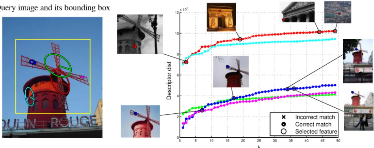
By definition, local features are regions which are distinctive. The matching score estimate the distinctiveness of detected local features by using descriptors. This is closer to practice where features are often accompanied by their descriptors.

The idea is to generate a set of tentative correspondences_Tdusing the descriptor similarity

measure DSIM_,_T_d _{as follows:}

Tm=SM(F(I)×F(J),DSIM)∩ Tr (3.6)

Note, that the features must be one-to-one matched not only by their descriptor distances but also by their region overlaps1. Because there are no constrains on the minimal similarity between descriptors, the search space cannot be pruned which makes the computation of this measure rather slow.

For SIFT descriptors the similarity measure is negative Euclidean distance:

DSIM_{(a, b) =}_−kD_(a)₋D_(b)_k _(3.7) MappingD:I(Ω)_→Rdstands for a descriptor of frameawheredis a descriptor length. Contrary to this definition, in some articles ([38]) the tentative correspondences are com-puted only as:

Tm′ =SM(F(I)×F(J),DSIM) (3.8)

i.e. that only descriptor distances are matched.

The matching score is based on the region descriptors, thus to compute the frame over-lap we use the measurement region which was used for descriptor calculation. We define MROverlap_{(a, b, ν), measurement region overlap as:}

MROverlap_{(a, b, ν) =} ΩΣaν2,x_a∩Ω_HT_Σ_b_ν2_H,Hxb ΩΣaν2,x_a∪Ω_HT_Σ_b_ν2_H,Hxb

(3.9) Usually the measurement regions size is set toν = 3. The threshold on maximal overlap error is set to constantǫ0m= 50% and the correspondences are obtained as:

(a, b)_{∈ C}m ⇐⇒ (a, b)∈ Tm, 1−MROverlap(a, b, ν)< ǫ0m (3.10)

Matching score is then computed using Equation 3.1. 1

This fact is not directly mentioned in the original article, however we have observed this when we have tried to reproduce the results from this article.

(32)

Figure 3.1: Categorisation of local image features in the descriptor benchmark from classi-fication perspective. True Positives (TP) together with False Negatives (FN) are features with sufficient overlap whereas matches are pairs whose descriptor distance is smaller than a threshold.

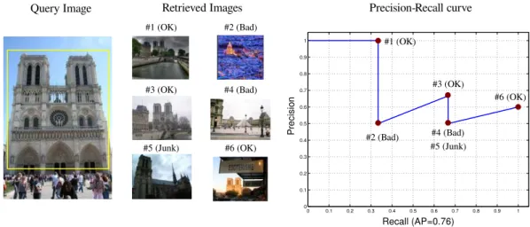
3.2 Evaluation of feature descriptors

The previous benchmark has been designed mainly for testing local image feature detectors. For testing the descriptors, Mikolajczyk and Schmid [28] propose slightly different framework which tests the image descriptors from an image classification perspective where the goal of the classifier is to classify each pair of image patches using image descriptors. It uses the same datasets as the benchmark for testing detectors which means that the ground truth is defined with homography between a reference imageIand testing image J.

For pair of imagesI, J, related with a homographyH, the input data for the classification is a set of ordered pairs of image framesX,X ⊆F(I)×F(J) with labelsY:{1,−1}where for x∈ X, x= (a, b) label y= 1 signifies that Overlap_{(a, b)}_>₁₋_ǫ_d _or_y ₌₋_{1 otherwise and} ǫd is maximal overlap error. The task is to classify whether the pair of image frames are in

correspondence (positive sample) or are not corresponding, i.e. to find function Classify_:

X → Ybased only on descriptors of the image frames.

The pairsx= (a, b) with labely= 1 are called correspondences (possible correct matches) and pairs where Classify_{(x) = 1 are in the former article called matches, see Figure 3.1.} There are several variants of this benchmark described in [28] which differ in the matching strategies:

Threshold-based matching In case of threshold based matching the classification is done

simply as:

Classify_tb_{(a, b) =} (

1 if_kD_(a)₋D_(b)_k_{< t}

−1 otherwise (3.11)

Wheretis descriptor distance threshold. Correspondences are all frame pairs which fulfil the overlap condition 3.11.

Nearest-neighbours matching In case of nearest-neighbour matching, the classification

function is defined as: Classify_nn_{(a, b) =}    1 ifb= arg min bi∈F(J) kD_(a)₋D_(b_i₎_{k ∧ k}D_(a)₋D_(b)_k_{< t} −1 otherwise (3.12)

This classification function achieves higher precisions as the particular value of descriptor distances varies with image transformations. The nearest neighbours matching classifies as a match only the closest descriptor below the threshold so there is smaller number of false

(33)

Figure 3.2: Visualisation of viewpoints per categories in DTU Robot dataset [1].

matches [29, p. 1622]. Because for each frame from the reference image there can be only one nearest neighbour, the set of correspondences is also defined differently, i.e. as a subset of matches where the frames fulfil the overlap criterion.

Second closest matching The second closest matching strategy extends the nearest

neigh-bour strategy with a test, whether the distance ratio of the second closest and the closest de-scriptor is under some threshold. It rejects matches which are too ambiguous. This strategy has been proposed by [24]. The set of correspondences is the same as for nearest-neighbour matching strategy.

The performance of the classifier is visualised with a precision-recall curve varying the threshold of descriptor distancest. The precision and recall is defined as follows (for details how positives and negatives are defined see Figure 3.1):

Precision = #TP #TP + #FP = #Correct matches #Matches (3.13) Recall = #TP #TP + #FN = #Correct matches #Correspondence (3.14)

In the original article, the PR curve is slightly modified so that onx-axis is 1₋Precision and on y-axis is Recall as the PR curve drawn in this way is more intuitive to read and is similar to the curves produced by the repeatability test.

3.3 DTU Robot 3D benchmark

DTU Robot 3D evaluation is a benchmark, proposed in [1], which compares the geometric precision of feature detectors. Contrary to homography benchmarks, ground truth is defined by a dense 3D stereo maps, which allows to find correspondences of points also in non-planar scenes. The dataset was acquired with a camera mounted on an industrial robot hand which provides very accurate camera positioning. Then the 3D model of the scene surface has been computed using structured light (the structured light does not affect the image data). The dataset contains 60 scenes of various objects (from model houses to fabric and vegetables) in 119 camera positions and 19 individual LED lightning. Camera positions are visualised in 3.2 and are grouped into three horizontal arcs and one linear path. All images are of resolution 1600_×1200px.

The correspondences are obtained based on three criteria which are visualised in Figure 3.3. Having a pair of image frames (a, b), a∈F_{(I), b}_∈F_(J_{), it is a valid correspondence when it} fulfils the following conditions:

(34)

(a) _(b)

(c)

Figure 3.3: Criteria for correspondences in DTU Robot dataset [1].

Reprojection error From the known camera positions and camera matrices, the 3D point

can be triangulated from the local feature centroid xa and xb. The triangulation is

computed using the linear solution produced by SVD [14, p. 312] (which minimises al-gebraic error) and the geometric reprojection error is further optimised using Levenberg-Marquardt algorithm [14, p. 314] to obtain optimised positions ˜xa and ˜xb. The

repro-jection error is then calculated as:

RepErr_{(a, b) =}_k_x_a₋_x_˜_a_k2₊_k_x_b₋_˜_x_b_k2 _(3.15) Frame pair (a, b) is a correspondence when:

(a, b)_{∈ A ⇐⇒} RepErr_{(a, b)}_{< ǫ}_rep _(3.16) Whereǫrep is maximal reprojection error usually set toǫrep= 2.5px.

Consistence with scene surface In this criterion the 3D surface reconstruction is used. In

order to decide whether a pair of frames (a, b)∈ B, the frame centrexais reprojected

onto a scene surface. Then a box of size 3mm in the scene is reprojected to the tested image and the correspondence is correct only whenxb lies in this reprojected box.

Absolute scale consistence This condition tests whether the frame scales are consistent.

It is fulfilled only when:

(a, b)_{∈ C ⇐⇒} max _σ′ a σ′ b ,σ ′ b σ′ a <2 (3.17)

(35)

Chapter

4

Improvements to VLBenchmarks project

In this chapter we describe our contribution to VLBenchmarks project. It has been mainly motivated by the necessity of having easy and fast benchmark software to assess the perfor-mance of various detectors and compare the results to the other state-of-the-art detectors.

Early version of the VLBenchmarks project, including parts presented in this work (Ho-mography and Retrieval benchmark), has been presented at ECCV 2012 in Florence as a part of the tutorialModern features: advances, applications, and software1_.

In this chapter we introduce the VLBenchmarks project and the state of the project before our commitment. Then we follow with implementation details and improvements of particular benchmarks. Among these benchmarks are two new benchmarks which has been newly introduced (epipolar benchmark and retrieval benchmark).

4.1 VLBenchmarks

VLBenchmarks is a project implemented in Matlab and originally developed by Varun Gul-shan and Andrea Vedaldi. Its main goal is to gather several benchmarks of computer vision algorithms. The former version implemented only computation of the repeatability score of local image feature detectors, see Section 3.1 for details. It contained wrappers for the original evaluation protocol by Kristian Mikolajczyk and some basic management structures to down-load detector binaries. It is important to note that the repeatability test implemented was several times faster than the original implementation however yielded rather different results than the KM test. The code of the original version is still available in public repository 2_{. In}

our implementation the overall structure and most of the original code has been changed. We have extended this project with additional tests. First, we have implemented matching score computation from [29] and created a versatile framework which allows to easily include new datasets, features extractors and evaluation benchmarks. Second, we have implemented novel direct evaluation of feature detectors and descriptors for image retrieval (further de-noted as retrieval benchmark) which mainly tests the distinctiveness of the detected regions and their descriptors. Another frequent use-case of interest region detectors is in 3D scene reconstruction pipelines where the precision of the feature location is crucial. For these cases we have implemented simple epipolar geometry test where we measure number and ratio of true correspondences in the set of tentative correspondences. The software was available as an open source project, Anders Boesen Lindbo Larsen had contributed by including the DTU Robot benchmark into the VLBenchmarks projects, which uses much more detailed ground truth data than our epipolar geometry benchmark.

Finally we have extended the project with the tests proposed in [28] for testing the local image features descriptors. Originally this test is limited for homography ground truth but it was extended to use the epipolar geometry ground truth.

1

https://sites.google.com/site/eccv12features/home 2

Czech Technical University in Prague Faculty of Electrical Engineering MASTER S THESIS. Karel Lenc