MODELING AND SIMULATION OF GRID CONNECTED PHOTOVOLTAIC DISTRIBUTED GENERATION SYSTEM

(1)

APPLICATION OF FUZZY CLUSTERING IN MULTI-SENSOR

INFORMATION FUSION

1

AIHONG TANG, 2YOUMEI ZHANG

1

College of information, mechanical and electrical engineering, Shanghai Normal University, Shanghai 200234, China

2

Department of Equipment and laboratory management, Shanghai Normal University, Shanghai 200234, China

ABSTRACT

In this article, we describe two kinds of Fuzzy clustering algorithm based on partition, use multiple sensors to collect valid data and classifies them. Fuzzy C-means algorithms are on the basis of the Hard C-means algorithm, and get a big improvement, making large data similarity as far as possible together. As a result of Simulation, FCM algorithm has more reasonable than HCM method on convergence, data fusion, and so on.

Keywords: Fuzzy Clustering, HCM, FCM 1. INTRODUCTION

In recent years, multi-sensor information fusion has made great achievements, has been applied to many aspects of the military and non-military. Multi-sensor information fusion unified the observation target or events from multiple sensors, under certain criteria, analysis and integrates to complete the comprehensive decision-making and the estimated task.

With the rapid development of robot technology, the robot's capabilities and the application has been enhanced. Intelligent robots is becoming the trend, while the sensor technology is the basis of the intelligent robot, intelligent robot is usually equipped with a number of different types of sensors in order to meet the needs of detection and data acquisition.

Due to the use of the information obtained by the single sensor has its limitations, the only binding part of the environmental characteristics of the information, leading to the uncertainty of the observations of the system, and it may be cause a system failure. The multi-sensor information fusion technology solves this problem effectively. In short, information fusion is the process of combining information and information obtained from the multi-sensor.

2. FUZZY CLUSTERING

Cluster analysis is an unsupervised pattern recognition method. Clustering is a data packet, and each group is referred to as a cluster. The data in

each cluster is called an object. The purpose of clustering is as similar as possible to the characteristics of the cluster object. The different characteristics of the different clusters in the object are as large as possible.

Traditional clustering analysis is a hard division, which is to divide each object to a class strictly, so this classification is demarcated. In fact, the boundaries between things are not distinct, there is the phenomenon of fuzzy partition. In 1965, the U.S. control theorist, mathematician, Zadeh published a paper 《Fuzzy sets》, proposed fuzzy set theory. The fuzzy set is applied to traditional clustering, the membership in the dataset object is represented with the membership function, the membership of each group is a value between in the continuous interval [0,1], with varying degrees of belonging to any cluster, rather than 0 or 1. The advantages of fuzzy clustering can be adapted to the data whose separation is not very good, and provide detailed information for the data structure description.

There are many clustering classification method: based on division, based on density, based on hierarchical, and so on. This paper only discusses the classification based on partition, including Hard-C means algorithm and Fuzzy C means algorithm.

2.1 Hard C-Means Algorithm（HCM）

(2)

choose C model feature vector as the initial cluster centers. Secondly, the data is classified into one of C class by the principle of division of the minimum distance one by one, then generate a new cluster. Finally, calculate the new various class centers after re-classification .As a result of the adjusted average calculated the center of all class, and as the C class, so called C-means method. HCM procedure is as follows:

Initialization: Given a cluster number of categories C, 2 ≤ C ≤ N, N is the number of data, μik is membership function, dik is the Euclidean

distance between No.k cluster center and No.i data point, set the iteration stop threshold ε, initialize the clustering prototype model PO, set the iteration

counter b = 0:

Step one: use the following formula or update the partition matrix Ub:

{

}

( ) ( )

, b min b ,

ik ir

b ik

1 d d 1 r C

0

µ =  = ≤ ≤

 （）

（1）

Step two: Use the following formula update clustering prototype pattern matrix Pb +1:

( 1)

b 1 1

i

( 1)

1

P , 1, 2,...,

N b ik k N b ik k xk i c µ µ + + = + = ⋅ =

∑

=

∑

（） (2) Step three: If ( )b (b 1)

i i

P −P + <ε , then the

algorithm stops and outputs the partition matrix u and the cluster prototype P, or let b = b +1, go to step one. Where • is some suitable matrix norm.

2.2Fuzzy C-Means Algorithm (FCM)

FCM clustering algorithm is one of the widely applied algorithms in unsupervised model recognition fields．As well-known，the optimal solution of FCM algorithm is obtained by minimizing the objective function.FCM clustering starts with selecting C initial clustering centers randomly (C is the number of clusters) and continue the algorithm by looping.FCM clustering is not perfect，either.Before using it，people need to know the number of clusters and good selection of initial cluster centers．If bad initial centers are picked，the objectire function of FCM algorithm will not go to a minimum value．

FCM algorithm is a clustering algorithm based on partition, the idea is: to make the object from the same cluster has best similarity, and the minimum

similarity between different clusters. FCM is based on HCM,using the fuzzy partition matrix and the fuzzy coefficient m, making further trimmed on the data classification, the calculation of the class center and the objective function.

FCM flow chart as follows figure 1: FCM procedure is as follows:

Initialization: Given a cluster number of categories C, 2 ≤ C ≤ N, N is the number of data, m is a fuzzy weighted index (m ∈ [1, ∞]), control the membership matrix of fuzzy, if m = 1, then the algorithm will be close of HCM. If m is greater, the object in each cluster membership will be smooth, Bezdek[1] gives an experience range 1≤m

≤5; Then derived from the physical interpretation, m = 2 is the most significant.Set the iteration stop

threshold value £, clustering the prototype model initialization PO, set the iteration counter b = 0: Step

one: Use the following formula or update the partition matrix Ub:

For ∀i，k，if ( )

0

b ik d

∃ > ，there is

1 2

( ) 1

( ) ( ) 1 b m C b ik ik b j jk d d

µ

− − =         =  __ _ _  __  __  

∑

(3) For ∀i，k，if

∃

d

_ik( )b

=

0

, there is

( )

1

b ir

µ

=

and for

j

≠

r

，

µ

_ij( )b

=

0

Step Two: Use the following formula update the clustering prototype pattern matrix Pb +1:

( 1)

b 1 1

i

( 1) 1

P , 1, 2, ...,

N b ik k N b ik k xk i c µ µ + + = + = ⋅ =

∑

=

∑

（）（4）

Step Three: If ( ) ( 1) £

b b i i

P −P + < , then the

(3)

Collect data

Determine C

Initialization cluster center

Calculation membership

Update cluster center

Stop Start

( ) ( 1)

£

b b

i i

P −P + <

No

Yes

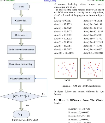
[image:3.612.89.527.82.597.2]

Figure.1. FCM Flow Chart

3. SIMULATION

The sensor is the robot's sensory and multi-sensor information fusion technology hardware base. An intelligent robot are usually equipped with hundreds of sensors. The sensor performance will directly affect the multi-sensor information fusion technology. For example, Using an intelligent robot, taking Microsoft Visual Basic 6.0 as experimental background, the robot with a variety

of sensors, including vision, torque, speed, temperature and so on.

In this case,the same random number 20, HCM and FCM were used to classify the two algorithms, take C = 3, result of the program as shown in figure 2:

(1) 59.2617 (2) 87.7273 (3) 82.9820 (4) 90.3477 (5) 80.8002 (6) 72.8252 (7) 59.1218 (8) 48.9351 (9) 98.0487 (10) 110.7192

data data data data data data data data data data

= = = = = = = = = =

(11) 46.0822 (12) 20.8139 (13) 63.0761 (14) 121.0287 (15) 22.4398 (16) 47.1740 (17) 112.5917 (18) 47.1393 (19) 63.6620 (20) 105.2211

data data data data data data data data data data

= = = = = = = = = =

HCM FCM

Figure. 2 HCM and FCM Classification

In figure 2,there are several different in it,as follows:

3.1 There Is Difference From The Cluster Center:

H.center(1,1)=38.7641 H.center(1,2)=0.0000 H.center(2,1)=71.1820 H.center(2,2)=0.0000 H.center(3,1)=106.3262 H.center(3,2)=0.0000

F.center(1,1)=56.4139

F.center(1,2)=0.0000

F.center(2,1)=21.6516

F.center(2,2)=0.0000

F.center(3,1)=100.5372

(4)

[image:4.612.98.510.73.708.2]

TABLE 1: HCM AND FCM

HC M

first class（

8,11,12,15,16,18）

48.9351,46.0822,20.8139,22.4398,47.1740,47.1393

second class（

1,2,3,5,6,7,13,19）

59.2617,87.7273,82.9820,80.8002,72.8252,59.1218,63.076 1,63.6620

third class （

4,9,10,14,17,20）

90.3477,98.0487,110.7192,121.0287,112.5917,105.2211

FCM

first class（

1,6,7,8,11,13,16,18,1 9）

59.2617,72.8252,59.1218,48.9351,46.0822,63.0761,47.174 0,47.1393,63.6620

second class（12,15） 20.8139,22.4398 third class（

2,3,4,5,9,10,14,17,20 ）

87.7273,82.9820,90.3477,80.8002,98.0487,110.7192,121.0 287,112.5917,105.2211

HCM

FCM

(5)

3.2 There Is Difference On The Basis Of The Cluster

FCM is based on membership classification; HCM is based on the distance from data to the cluster center.

1) FCM membership degree:

F.Degree(1,1)=0.9999

F.Degree(1,2)=0.0267

F.Degree(1,3)=0.1571

F.Degree(1,4)=0.0079

F.Degree(1,5)=0.2946

F.Degree(1,6)=0.8807

F.Degree(1,7)=1.0000

F.Degree(1,8)=0.9940

F.Degree(1,9)=0.0000

F.Degree(1,10)=0.0013

F.Degree(1,11)=0.9682

F.Degree(1,12)=0.0000

F.Degree(1,13)=0.9983

F.Degree(1,14)=0.0101

F.Degree(1,15)=0.0000

F.Degree(1,16)=0.9825

F.Degree(1,17)=0.0021

F.Degree(1,18)=0.9821

F.Degree(1,19)=0.9976

F.Degree(1,20)=0.0001

F.Degree(2,1)=0.0000 F.Degree(2,2)=0.0014 F.Degree(2,3)=0.0056 F.Degree(2,4)=0.0005 F.Degree(2,5)=0.0086 F.Degree(2,6)=0.0094 F.Degree(2,7)=0.0000 F.Degree(2,8)=0.0055 F.Degree(2,9)=0.0000 F.Degree(2,10)=0.0002

F.Degree(3,1)=0.0000

F.Degree(3,2)=0.9719

F.Degree(3,3)=0.8373

F.Degree(3,4)=0.9916

F.Degree(3,5)=0.6969

F.Degree(3,6)=0.1099

F.Degree(3,7)=0.0000

F.Degree(3,8)=0.0004

F.Degree(3,9)=1.0000

F.Degree(3,10)=0.9986

(6)

H.Degree(1,1)=421.1521 H.Degree(1,2)=2398.4021 H.Degree(1,3)=1956.2284 H.Degree(1,4)=2661.8729 H.Degree(1,5)=1768.0384 H.Degree1,6)=1161.1630 H.Degree(1,7)=415.4389 H.Degree(1,8)=104.4502 H.Degree(1,9)=3515.6737 H.Degree(1,10)=5178.5356

H.Degree(1,11)=54.5554

H.Degree(1,12)=323.2081

H.Degree(1,13)=592.0747

H.Degree(1,14)=6768.4788

H.Degree(1,15)=267.4804

H.Degree(1,16)=71.7278

H.Degree(1,17)=5451.5245

H.Degree(1,18)=71.1439

H.Degree(1,19)=620.9056

H.Degree(1,20)=4417.5361

H.Degree(2,1)=143.0953 H.Degree(2,2)=274.7466 H.Degree(2,3)=140.2395 H.Degree(2,4)=368.3227 H.Degree(2,5)=93.5092 H.Degree(2,6)=3.7000 H.Degree(2,7)=146.4487 H.Degree(2,8)=495.9262 H.Degree(2,9)=722.8195 H.Degree(2,10)=1564.1830

H.Degree(3,11)=3630.3367

H.Degree(3,12)=7313.3516

H.Degree(3,13)=1871.5717

H.Degree(3,14)=217.1651

H.Degree(3,15)=7037.9217

H.Degree(3,16)=3499.9772

H.Degree(3,17)=40.2569

H.Degree(3,18)=3504.0938

H.Degree(3,19)=1821.2366

H.Degree(3,20)=2.2213

3.3 Result Of Classification

Figure 2 shows a little different from the classification between them, specific classification, such as table 1 .

Through above experience, In FCM clustering algorithm, Appling the maximum membership degree method, data in each class is reasonable, it can make big similarity of the data together.

4. CONCLUSION

HCM algorithm divides each sample to one category directly, FCM algorithm achieves the division of a given sample set by the objective function through iterative optimization algorithm. it can represent membership degree that the points belong to different categories. The classification as follows figure 3.

(7)

many shortages, such as the choice of initial cluster centers, whether the random number with cluster structure to be studied further.

In short, information fusion is a field of study, it provides for combining pieces of information from the different sensors, resulting in improved overall system performance, reliability, with respect to a separate sensor. Information fusion method has been developed to optimize the output of the entire system is useful in a variety of applications of data fusion: security, medical diagnostics, environmental monitoring and remote sensing.

REFRENCES:

[1] Richard J. Hathaway and James C. Bezdek, “Recent convergence results for the fuzzy c-means clustering algorithms”, Journal of Classification, Vol. 5, No. 2, 1988, pp. 237-247

[2] Jian Xu, JianXun Li and Sheng Xu, “Data fusion for target tracking in wireless sensor networks using quantized innovations and Kalman filtering”, Science China Information Sciences, Vol. 55, No. 3, 2012, pp.530-544. [3] Jamal Ahmad Dargham, Ali Chekima, Sigeru

Omatu and Chelsia Amy Doukim, “Data fusion for skin detection”, Artificial Life and Robotics, Vol. 13, No. 2, 2008, pp. 438-441. [4] Levent Yenilmez and Hakan Temeltas, “A

new approach to map building by sensor data fusion: sequential principal component-SPC method”, The International Journal of Advanced Manufacturing Technology, Vol. 34, No. 1-2, 2007, pp. 168-178.

[5] Zhong Li, “Fuzzy Logic and Fuzzy Control Studies in Fuzziness and Soft Computing”, Fuzzy Chaotic Systems, Vol. 199, 2006, pp.13-29.

[6] Min Liu, Yi Zhuang, “Multi-target Tracking Algorithm Based on Fuzzy C-Spherical Shells”, Computer Engineering, Vol. 37, 2011, pp.201-204.

[7] Haijun Wang, Yu Deng, Jia Liu, “Spatial Clustering Method based on Fuzzy C-mean”, Journal of Hua Zhong Normal University, Vol. 43, No. 1, 2009, pp. 152-155.

[8] Kevin J. Johnson, Christian P. Minor, Verner N. Guthrie and Susan L. Rose-Pehrsson, “A Study on Feasibility of Integrating Probe Vehicle Data into A Traffic State Estimation Problem using Simulated Data”, Stochastic

Environmental Research and Risk Assessment, Vol. 23, No. 2, 2009, pp. 237-252.