Numerical Solution of Higher Order Linear Fuzzy Differential Equations using Generalized STWS Technique

(1)

ISSN(Online) : 2319-8753 ISSN (Print) : 2347-6710

I

nternational

J

ournal of

I

nnovative

R

esearch in

S

cience,

E

ngineering and

T

echnology

(An ISO 3297: 2007 Certified Organization)

Vol. 5, Issue 3, March 2016

Numerical Solution of Higher Order Linear

Fuzzy Differential Equations using

Generalized STWS Technique

Emimal Kanaga Pushpam A1, Anandhan P 2

Associate Professor, Department of Mathematics, Bishop Heber College, Tiruchirappalli, Tamil Nadu, India1

Assistant Professor, Department of Mathematics, Ganesar College of Arts and Science, Pudukkottai, Tamil Nadu,

India2

ABSTRACT: This paper presents the numerical solutionofhigher order linear fuzzy differential equations(FDEs)

using generalized Single Term Walsh Series Technique (STWS). The applicability of this technique is illustrated by examples. The numerical results are compared with their exact solutions.

KEYWORDS:Fuzzy differential equations, linear system, IVP, Generalized STWS.

I. INTRODUCTION

Recently the study of fuzzy differential equations has been growing rapidly. The fuzzy derivative was introduced by Chang andZadeh[1].Seikkala and Kaleva have studied Fuzzy IVPs[2 - 4].Further many researchers have suggested various numerical methods for solving fuzzy differential equations[5-9].

STWS technique was introduced by Rao et al. [10]. Balachandran and Murugesan applied STWS technique to solve first order system of IVPs[11, 12]. Murugesan and Paul Dhayabaran extended STWS technique for solving second order singular system of IVPs[13]. Emimalet al.[14] proposed the generalized STWS Technique to solve system of IVPs of any order ‘n’ with ‘p’ variables.

In this paper we adopt this generalized STWS technique to solve higher order linear fuzzy IVPs. In Section 2, we provide definitions and results on fuzzy numbers and fuzzy derivatives. In Section 3, we define fuzzy Cauchy problem. In Section 4, we give the generalized Single Term Walsh Series Technique which is capable of determining the discrete solutions of the linear systems of IVPs of any higher order ‘n’ with ‘p’ variables. In Section 5 we provide numerical examples to illustrate the applicability of the generalized STWS technique in solving fuzzy IVPs.

II. PRELIMINARIES

According to Zadeh, a fuzzy set is a generalization of classical set that allows membership function to take any value in the unit interval [0,1].

Definition 1

Let A be a fuzzy set defined in R. A is called a fuzzy interval if

1. A is normal, that is there exists x₀Rsuch that A x( ₀)1

2. A is convex, that is for all ,x yR and 01, it holds that

( (1 ) y min(A(x), A(y)

Ax  

3. A is upper semi-continuous, that is for any x₀Rit holds that

0 0

( ) lim ( )

x x

A x A x

 

(2)

I

nternational

J

ournal of

I

nnovative

R

esearch in

S

cience,

E

ngineering and

T

echnology

4. 0

[ ]A {xR/ ( )x 0}is a compact subset of R.

Definition 2

Let A be a fuzzy interval defined in R. The α- cut of A is the set [A]that contains all elements in R such that the

membership values of A is greater than or equal to α, that is

[A]{xR/ A( )x }, (0,1].

For a fuzzy interval A, it’s α- cut are closed intervals in R and we denote them by

[A]_[A , A ],  __(0,1].

Definition 3

A fuzzy interval A is called a triangular fuzzy interval if its membership has the following form

0,

, A ( )

,

0,

if x a x a

if a x b b a

x

c x

if b x c c b

if x c

 

 

  

   



 _ _

 

 _



and its α-cuts are simply[A] [a (b a), c (c b)], (0,1].

  

      It is clear that

1. Ais a bounded left continuous non decreasing function over [0,1] ,

2. Ais a bounded right continuous non increasing function over[0,1],

3. A A  [0,1].

Definition 4

The supremum metric

d

 on E is defined by d ( , )U V sup{d [ ] ,[ ] ) :HU V I},

  _

   and(E d, ) is a complete metric

space.

Definition 5

A mapping F I: E is Hukuhara differentiable at t₀T R if for some h₀ 0 the Hukuhara difference

0 0 0 0

( ) ~_h ( ), ( ) ~_h ( ),

F t  t F t F t F t  t

exist in E for all0  t h₀ and if there exists an

F t

'

( )

₀



E

such that '

0 0

(F(t ) ~ ( ))

lim h ( ) 0

t

t F t

d F t

t

   

 

 

 and

'

0 0

(F(t ) ~ ( ))

lim h ( ) 0,

t

F t t

d F t

t

   

 

  

the fuzzy set is called the Hukuhara derivative of F at t0.

Definition 6

The fuzzy integral

( ) dt, 0 a b 1

b

a

y t   



isoutlined by

( ) ( ) , ( )

b b b

a a a

y t dt y t dt y t dt



 

   



   





 





provided the Lebesgue integrals on the proper exist.

Definition 7

(3)

I

nternational

J

ournal of

I

nnovative

R

esearch in

S

cience,

E

ngineering and

T

echnology

The Seikkala derivative

y t

'

( )

of a fuzzy process y is defined by

' ' '

[ ( )]y t  [(y) ( ), (t y) ( )], 0t 1,provided by this equation defines a fuzzy number

y t

'

( )



E.

III. FUZZY INITIAL VALUE PROBLEM

Consider the fuzzy initial value problem in the following form:

0

0 0

'( ) ( , ( ), [ , ]

( )

y t f t y t t t T

y t y

 

 

 

wherey is a fuzzy function of t, f(t, y) is a fuzzy operation of the crisp variablet and the fuzzy variable y,

y

'

is

the fuzzy derivative of y and y(t0) = y0 is afuzzy number. Therefore we have a fuzzyCauchy problem.

We denote the fuzzy function y by [ , ]y y . It means that the α-level setof y(t) for t[ , ]t T₀ is

0 0 0

[ ( )]y t [ ( ; ),y t  y t( ; )], [ ( )]y t [ ( ; ),y t y t( ; )], (0,1].

By using the extension principle of Zadeh, we have the membership function

( , ( ))( ) sup{ ( )( ) | ( , )},

f t y t s  y t  f t sR

so ( , ( ))f t y t is a fuzzy number. From this it follows that

[ ( , ( ))]f t y t  [ ( , ( ); ),f t y t  f t y t( , ( ); )], (0,1] where

( , ( ); ) min{ ( , ) / [ ( ; ), ( ; )]

( , ( ); ) max{ ( , ) / [ ( ; ), ( ; )] f t y t f t u u y t y t

f t y t f t u u y t y t

  

 

We define

( , ( ); ) [t, ( ; ), ( ; )], ( , ( ); ) [t, ( ; ), ( ; )]. f t y t  F y t y t f t y t  G y t y t

In this paper we solve higher order linear system of fuzzy IVPs using STWS technique. Consider an nth order linear

system of fuzzy differential equations of the form

A0 X(n) (t) = A1X(n – 1) (t) + A2 X(n – 2 ) (t) + . . . + An -1X(1)(t)+ AnX( t ) + Bu(t)

withX(0) = X0 and X( j ) (0) = X0(j) , j = 1, 2, … (n-1)

where A0, A1, . . ., An



Rpx p, B



Rpxr, X(t) is the p-state vector, u(t) is an r-input vector.

HereX( )j is the jthderivative of X, X0’s are fuzzy numbers and X’s are fuzzy variables.

IV. GENERALIZED STWS TECHNIQUE FOR SOLVING LINEAR TIME INVARIANT SYSTEMS [14]

Consider an nth order time-invariant linear system of the form

A0 X(n) (t) = A1X(n – 1) (t) + A2 X(n – 2 ) (t) + . . . + An -1X(1)(t)+ AnX( t ) + Bu(t)

with X(0) = X0 and X( j ) (0) = X0(j) , j = 1, 2, … (n-1) (1 )

where A0, A1, . . ., An



Rpx p, B



Rpxr, X(t) is the p-state vector, u(t) is an r-input vector.

Here ( )j

X is the jthderivative of X.

The nthorder system given by Eqn. (1) is called a singular system while A0 is singular. The given functions are

multiplied as a single term Walsh series in the normalized interval s [0,1) which corresponds to t  [0, 1/m) by

defining t = s/m, m being any integer. Within the normalized interval, Eqn. (1) becomes

) ( ) ( )

( ...

) ( )

( )

( (1)

) 1 (

) 1 ( )

2 ( 2 2 ) 1 ( 1 ) (

0 u s

m B s X m

A s X m

A s

X m

A s X m A s X

A n_n _n

n n n

n n

 

  

   _ (2)

Expressing Eqn. (2) in STWS with

X( n – j ) ( s ) = (Cj) i(s) , (j =0, 1, 2, …, n – 1) X (s) = (Cn) i(s)

(4)

I

nternational

J

ournal of

I

nnovative

R

esearch in

S

cience,

E

ngineering and

T

echnology

where Cj’s (j =0, 1, 2, …, n – 1) are BPF values of nth rate, (n-1)th rate, … , 1st rate, state and input vector respectively

in s  [0,1), the following set of recursive equations with the operational matrix for integration E =

2 1

has been

obtained:

1

1 2 n

1 i 0 2 n

(n-j 1) i (j-1) i

(n-j) (n-j)

j i

n i

A A A

(C ) A - - - ... - G 2m (2m) (2m)

1

( ) (C ) X (i-1) , (j 2, 3, ..., n) 2

X ( i ) (C ) X (i-1) , (j 1, 2, ..., (n-1) )

X(i) (C ) X(i-1)

i

j C





 

  

 

  

 

(3)

where

(n-1) 3 (n-2)

1 2 n 2

2 ( 1) n 2 3 ( 2)

A

A A A A

... X (i-1) ... X (i-1)

m 2m 2 m 2m 2

n

i n n n

A G

m m

 

 

 _   _  _   _

   

n

i

n n

A B

... X(i-1) H

m m

   andi = 1, 2, 3, . . . .

Using these recursive equations, the discrete values of X, X(1) , X(2) ,…, X(n-1) in Eqn. (1) can be determined with the

initial conditions.

These equations give solutions for all integer values of ‘m’. In the case of singular system, that is, if A0 is singular, the

matrix

1 2 n

0 2 n

A A A

A - - - ... 2m (2m) (2m)

 

 

 

becomes non-singular, which is an added advantage of this method. The value of ‘m’ may be decided on large enough to growth the accuracy of results.The STWS approach is rather solid because it's far based totally on the Trapezoidal rule, that's an A-stable approach.

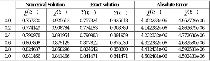
V. NUMERICAL EXAMPLES Example 1

Consider the second order fuzzy differential initial value problem "( ) ( ), [0,1]

(0) 0

' (0) [0.9 0.1 , 1.1 0.1 ], where 0 1. y t y t t

y

y   

  

 

 

 _ _ _ _ _



The exact solution is given by

( ; ) [(0.9 0.1 ) sin( ), (1.1 0.1 ) sin( )].

y t     t   t

The results are shown in the following Table 1 and Fig. 1.

Table 1 Results of Example 1 (at t = 1)

α

Numerical Solution Exact solution Absolute Error

( ; )

y t y t( ; ) Y t( ; ) Y t( ; ) y t( ; ) y t( ; )

0.0 0.757320 0.925613 0.757324 0.925618 4.052233e-06 4.952729e-06

0.2 0.774149 0.908784 0.774153 0.908789 4.142282e-06 4.862679e-06

0.4 0.790978 0.891954 0.790983 0.891959 4.232332e-06 4.772630e-06

(5)

I

nternational

J

ournal of

I

nnovative

R

esearch in

S

cience,

E

ngineering and

T

echnology

Fig. 1 Solution Graph of Example 1

Example 2

Consider the following fuzzy IVP

"'( ) 2 "( ) 3 ( ), (0 1)

(0) (3 , 5 ), '(0) ( 1 , 3 ), "(0) (8 , 10 )

y t y t y t t

y   y   y  

   

 

          



The exact solution is as follows:

3 3

1 7 11 1 7 19

( ; ) ,

3 12 4 3 12 4

t t t t

y t  e  e e  e

  _ _  _   _  _ _

   

 

α Numerical Solution Exact solution Absolute Error ( ; )

y t  y t( ; ) _{Y t}_{( ; )} Y t( ; ) y t( ; ) y t( ; )

0.0 12.394939 13.130698 12.394898 13.130657 4.105947e-05 4.096367e-05 0.2 12.468515 13.057122 12.468474 13.057081 4.104989e-05 4.097325e-05

0.4 12.542091 12.983546 12.542050 12.983505 4.104031e-05 4.098283e-05

0.6 12.615667 12.909971 12.615626 12.909930 4.103073e-05 4.099241e-05

0.8 12.689243 12.836395 12.689202 12.836354 4.102115e-05 4.100199e-05

1.0 12.762819 12.762819 12.762778 12.762778 4.101157e-05 4.101157e-05

12.3 12.4 12.5 12.6 12.7 12.8 12.9 13 13.1 13.2 13.3 0

0.1 0.2 0.3 0.4 0.5 0.6 0.7 0.8 0.9 1

Numerical Values

A

lp

h

a

V

a

lu

e

s

Comparision of STW S Solution and Exact Solution at t = 1, m = 800 S TW S E xact 0.74 0.76 0.78 0.8 0.82 0.84 0.86 0.88 0.9 0.92 0.94 0

0.1 0.2 0.3 0.4 0.5 0.6 0.7 0.8 0.9 1

Numeric al Values

A

lp

h

a

V

a

lu

e

s

(6)

I

nternational

J

ournal of

I

nnovative

R

esearch in

S

cience,

E

ngineering and

T

echnology

Example 3

Consider the following fourth Order fuzzy linear differential equation ( 4)

( ) 0, [0,1]

(0) ( 1, 1 ), '(0) ( 1, 1 ),

"(0) ( 1, 1 ), "' (0) ( 1, 1 )

y t y t

y r r y r r

    

      

 _ _ _ _ _ _ 

with the exact fuzzy solution

( ; ) ( 1) , (1t ) t .

y t r _ r e r e_

α Numerical Solution Exact solution Absolute Error ( ; )

y t  y t( ; ) Y t( ; ) Y t( ; ) y t( ; ) y t( ; )

0.0 -2.718304 2.718304 -2.718282 2.718282 2.265278e-05 2.265278e-05 0.2 -2.174644 2.174644 -2.174625 2.174625 1.812223e-05 1.812223e-05 0.4 -1.630983 1.630983 -1.630969 1.630969 1.359167e-05 1.359167e-05 0.6 -1.087322 1.087322 -1.087313 1.087313 9.061113e-06 9.061113e-06 0.8 -0.543661 0.543661 -0.543656 0.543656 4.530557e-06 4.530557e-06 1.0 0.000000 0.000000 0.000000 0.000000 0.000000e+00 0.000000e+00

Example 4

Consider the following system of first order fuzzy differential equations

1 2

2 1 2

1 2

'( ) ,

'( ) 4 4 , [0,1]

(0) (2 , 4 ), (0) (5 , 7 ) y t y

y t y y t

y r r y r r

  

   



 _ _ _ _ _ _



The exact solution is as follows:

2 2 2 2

1

2 2 2 2 2 2

2

( ; ) [(2 ) (1 ) t , (4 ) (r 1) t ]

( ; ) [(4 2 ) (1 ) (2 2 ) t , (r 1) (8 2 ) (2 2 ) t ]

t t t t

t t t t t t

y t r r e r e r e e

y t r r e r e r e e r e r e

      

          

The results of Y1are shown in the following Tables 4 and Fig. 4.

-3 -2 -1 0 1 2 3 0

0.1 0.2 0.3 0.4 0.5 0.6 0.7 0.8 0.9 1

Numerical Values

A

lp

h

a

V

a

lu

e

s

(7)

I

nternational

J

ournal of

I

nnovative

R

esearch in

S

cience,

E

ngineering and

T

echnology

Table 4 Results of Y1in Example 4 (at t = 0.7)

α Numerical Solution Exact solution Absolute Error 1( ; )

y t

1( ; )

y t Y t1( ; ) Y t1( ; ) y t1( ; ) y t₁( ; ) 0.0 10.949052 3.382165 10.949040 3.382160 1.241907e-05 5.322453e-06 0.2 11.192364 3.138854 11.192352 3.138848 1.170941e-05 6.032114e-06 0.4 11.435675 2.895543 11.435664 2.895536 1.099975e-05 6.741776e-06 0.6 11.678986 12.652231 11.678976 2.652224 1.029009e-05 7.451438e-06 0.8 11.922297 12.408920 11.922288 2.408912 9.580423e-06 8.161100e-06 1.0 12.165609 12.165609 12.165600 12.165600 8.870761e-06 8.870761e-06

Fig. 4 Solution Graph for Y1 of Example 4

The results of Y2 are shown in the following Tables 5 and Fig. 5.

Table 5 Results of Y2 in Example 4 (at t = 0.7)

α Numerical Solution Exact solution Absolute Error 2( ; )

y t

2( ; )

y t Y t2( ; ) Y t2( ; ) y t2( ; ) y t₂( ; ) 0.0 25.953308 22.709128 25.953280 22.709120 2.779506e-05 7.687984e-06 0.2 25.628890 23.033546 25.628864 23.033536 2.578435e-05 9.698692e-06 0.4 25.304472 23.357964 25.304448 23.357952 2.377365e-05 1.170940e-05 0.6 24.980054 23.682382 24.980032 23.682368 2.176294e-05 1.372011e-05 0.8 24.655636 24.006800 24.655616 24.006784 1.975223e-05 1.573082e-05 1.0 24.331218 24.331218 24.331200 24.331200 1.774152e-05 1.774152e-05

Fig. 5 Solution Graph for Y2 of Example 4 10.50 11 11.5 12 12.5 13 13.5 0.1

0.2 0.3 0.4 0.5 0.6 0.7 0.8 0.9 1

STW S Solution and Exact Solution of Y1 at t = 0.7, m = 800

Numerical Values

A

lp

h

a

V

a

lu

e

s

STW S Exact

22.5 23 23.5 24 24.5 25 25.5 26 0

0.1 0.2 0.3 0.4 0.5 0.6 0.7 0.8 0.9 1

STWS Solut ion and Exact S olution of Y2 at t = 0.7, m = 800

Numerical Values

A

lp

h

a

V

a

lu

e

s

(8)

I

nternational

J

ournal of

I

nnovative

R

esearch in

S

cience,

E

ngineering and

T

echnology

VI. CONCLUSION

In this paper, the generalized STWS method has been adopted to solve the linear systems of fuzzy IVPs. The effectiveness of this approach has been illustrated via examples. The numerical outcome had been compared with exact solutions. From the tables, it is observed that the absolute error is negligibly small. This suggests that the generalized STWS technique is suitable for linear systems of fuzzy IVPs of any order with any number of variables. Since STWS method is an A-Stable method, one can get the results for any length of time.

REFERENCES

[1] Chang S. L., and Zadeh L. A, “On Fuzzy Mapping and Control”, IEEE Trans. System Man Cybernet, Vol. 2,pp. 30-34, 1972. [2] Kaleva O., “Fuzzy Differential Equations”, Fuzzy Sets Systems, Vol, 24, pp. 301-317, 1987.

[3] Seikkala S., “On the Fuzzy Initial Value Problem”, Fuzzy Sets Systems, Vol, 24, pp. 319-330, 1987.

[4] Kaleva O., “The Cauchy problem for Fuzzy Differential Equations”, Fuzzy Sets Systems,Vol, 35, pp. 389-396, 1990.

[5]Abbasbandy S., AllahViranloo T., “Numerical solution of fuzzy differential equation by Taylormethod”, Journal of Computational Methods in Applied Mathematics, Vol. 2, pp. 113-124, 2002.

[6]Abbasbandy S., AllahViranloo T., “Numerical solution of fuzzy differential equation, Mathematical and Computational Applications”, Vol. 7, pp. 41-52, 2002.

[7]Abbasbandy S., AllahViranloo T., “Numerical solution of fuzzy differential equation by Runge-Kutta method”, Nonlinear Studies, Vol.11, pp. 117-129, 2004.

[8] Allahviranloo T., Ahmady N., Ahmady E., “Numerical solution of fuzzy differential equations by predictor-Corrector method”, Information Sciences, Vol. 177, pp. 1633-1647, 2007.

[9] Allahviranloo T., Abbasbandy S., Ahmady N., Ahmady E., “Improved predictor-Corrector method for solving fuzzy initial value problems”, Information Sciences, Vol. 179, pp. 945-955, 2009.

[10] Rao G.P., Palanisamy K.R., Srinivasan T., “Extension of computation beyond the limit of normal interval in Walsh series analysis of dynamical systems”, IEEE. Trans. Automat. Contr., Vol. 25, pp. 317–319, 1980.

[11] Balachandran K., Murugesan K., “Analysis of different systems via single term Walsh series method”, International Journal of Computer Mathematics, Vol. 33, pp. 171–179, 1990.

[12] Balachandran K., Murugesan K., “Analysis of non-linear singular systems via STWS method”, International Journal of Computer Mathematics, Vol. 36, pp. 9–12, 1990.

[13] Murugesan K., Dhayabaran D.P., Evans D.J., “Analysis of second order multivariable linear system using single-term Walsh series technique and Runge-Kutta method”, International Journal of Computer Mathematics, Vol. 72, pp. 367–374, 1999.