c
DISTRIBUTED OPTIMIZATION WITH APPLICATIONS TO SENSOR NETWORKS AND MACHINE LEARNING
BY
KUNAL SRIVASTAVA
DISSERTATION
Submitted in partial fulfillment of the requirements
for the degree of Doctor of Philosophy in Systems and Entrepreneurial Engineering in the Graduate College of the
University of Illinois at Urbana-Champaign, 2011
Urbana, Illinois
Doctoral Committee:
Assistant Professor Angelia Nedi´c, Chair
Associate Professor Duˇsan Stipanovi´c, Co-Director of Research Professor P. R. Kumar
Abstract
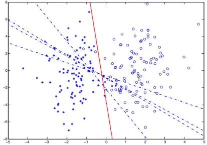
This dissertation deals with developing optimization algorithms which can be distributed over a network of computational nodes. Specifically we develop distributed algorithms for the special class when the optimization problem of interest has a separable structure. In this case the ob-jective function can be written as a sum of local convex obob-jective functions. Each computational node has knowledge of its own local objective function and its local constraint set and needs to cooperatively solve the optimization problem under this information constraint. Furthermore we consider the case when the communication topology of the nodes is dynamic in nature. Recently, there has been a lot of interest in the so called “consensus” algorithms which has been shown to be remarkable robust to dynamic communication topology. Our algorithms leverage the robustness properties of consensus algorithm to compute the optimal solution in a distributed manner. We propose algorithms which have guaranteed convergence behavior in the presence of various forms of perturbations like communication noise, stochastic subgradient errors and stochastic commu-nication topologies. This enables our algorithms to be useful in a wide class of application areas in sensor networks and machine learning. Specifically the consideration of stochastic subgradient errors enable our algorithms to be useful in an online setting, when the algorithm operates on streaming data. We adapt our algorithms for the binary classification problem in the support vector machine setting and show the behavior over a sample data set.
We further develop distributed algorithms for the min-max problem in a network. This formu-lation doesn’t readily fit the separable structure of the objective function discussed earlier. We develop an exact penalty based approach and an approach based on primal-dual iterative schemes. We show the applicability of the algorithms on a power allocation problem in cellular networks.
Acknowledgements
First and foremost I express my deep sense of gratitude to my advisors Professor Angelia Nedi´c and Duˇsan Stipanovi´c. They provided valuable guidance, motivation and support during the course of this research and have been great academic role models to look up to and emulate. I am also indebted to Professor Mark Spong for advising and supporting me during the early phase of my PhD. I would also like to thank Professor P.R. Kumar and Professor R.S. Sreenivas for serving on my doctoral committee.
I owe a great deal to all the wonderful teachers I had at University of Illinois. They have helped me develop tools which have held me in good stead. A special thanks to Professor P.R. Kumar, Professor Daniel Liberzon, Professor Tamer Ba¸sar, Professor Sean Meyn and Professor Richard Sowers.
I had the good fortune of meeting a lot of wonderful people at CSL who made CSL an ideal research environment. In particular I would like to thank Hemant Kowshik, Jayakrishnan Un-nikrishnan, Arvind Ganesh, Jayanand Asok-Kumar, Anand Muralidhar, Ramakrishna Gummadi, Vijay Raman, Nikos Freris, Silvia Mastellone and Peter Hokayem. In addition I would like to thank Anil Kumar, Mamta Singh, Jagannathan Rajagopalan, Vivek Natarajan, Gayathri Mohan, Sophie Pwet, Anjan Raghunathan, Rajan Lakshmi Narasimha, Shankar Sivaramakrishnan, Karthik Jam-bunathan, Sreeram Kannan and Chaitanya Sathe for their friendship and helping me in various tangible and intangible ways.
My brothers Anurag and Neelabh have always been there despite the distance and finally my par-ents have been a pillar of strength providing me with their love, unwavering support and motivation and I owe all of this to them.
Table of Contents
Chapter 1 Introduction . . . 1
1.1 Problem Outline . . . 2
1.2 Statement of Contribution and Organization . . . 4
Chapter 2 Mathematical Preliminaries . . . 8
2.1 Notation and Terminology . . . 8
2.2 Bregman Distance . . . 10
2.3 Basic Results . . . 12
Chapter 3 Consensus Based Algorithm for Convex Feasibility Problems . . . 13
3.1 Successive Orthogonal Projection . . . 14
3.1.1 The Multiprojection Algorithm . . . 15
3.2 Problem Formulation . . . 16 3.2.1 Model Assumptions . . . 18 3.3 Preliminary Results . . . 19 3.4 Convergence Result . . . 22 3.5 Subspace Constraints . . . 23 3.6 Conclusion . . . 26
Chapter 4 Synchronous Algorithm for Distributed Constrained Stochastic Op-timization . . . 27
4.1 Incremental Subgradient Algorithm . . . 28
4.2 The Stochastic Optimization Problem . . . 29
4.3 Distributed Optimization Problems Arising In Networks . . . 29
4.3.1 Consensus and Robust Estimation . . . 30
4.3.2 Constrained Estimation . . . 30
4.3.3 Network Utility Maximization in a Wireless Network . . . 32
4.3.4 Distributed Model Predictive Control . . . 32
4.4 Main Algorithm . . . 34
4.4.1 Assumptions . . . 35
4.5 Preliminary Results . . . 36
4.6 Convergence Result . . . 41
Chapter 5 Asynchronous Algorithms . . . 44
5.1 Network Model, Outline of Algorithms and Assumptions . . . 46
5.1.1 Constrained Consensus: . . . 46
5.1.2 Distributed Optimization: . . . 48
5.1.3 Assumptions and Implications . . . 49
5.1.4 Gossip based communication protocol . . . 53
5.1.5 Broadcast based communication protocol . . . 54
5.2 Preliminary Results . . . 55
5.3 Constrained Consensus . . . 58
5.3.1 Convergence Result . . . 60
5.3.2 Constant step size error bound . . . 63
5.4 Distributed Optimization . . . 65
5.4.1 Preliminary results . . . 66
5.4.2 Convergence Result . . . 72
5.4.3 Constant step size error bound . . . 77
5.5 Conclusion . . . 82
Chapter 6 Distributed Bregman Distance Algorithms for Min-Max Optimization 83 6.1 Problem Formulation . . . 84
6.1.1 Problem Reformulation . . . 85
6.2 Exact Penalty Function Approach . . . 85
6.2.1 Equivalence Between Epigraph and Penalty Problem Formulations . . . 87
6.2.2 Algorithm . . . 88
6.2.3 Assumptions . . . 91
6.2.4 Preliminary Results . . . 93
6.2.5 Analysis of the Algorithm . . . 95
6.3 Primal-Dual Algorithm . . . 101
6.3.1 Analysis of the Algorithm . . . 102
6.4 Min-Max Game Against Exogenous Player . . . 109
6.4.1 Algorithm . . . 110
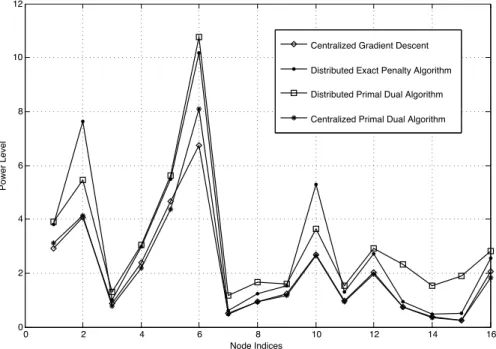
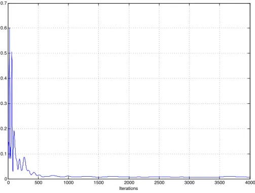
6.5 Uplink Power Control . . . 111
6.5.1 Simulation Result . . . 112
6.6 Conclusion . . . 112
Chapter 7 Application to Distributed Supervised Learning . . . 115
7.1 Supervised Learning Problem . . . 116
7.1.1 Batch Learning . . . 117
7.1.2 Online Learning . . . 119
7.2 Distributed Batch Learning . . . 120
7.2.1 Least-Squares Regression . . . 120
7.2.2 General Convex Loss Functions . . . 123
7.3 Distributed Online Learning in Parallel Data Streams . . . 129
7.3.1 Distributed Online Support Vector Machines . . . 129
7.4 Conclusion . . . 132
Chapter 1
Introduction
There has been a sustained effort in the research community over the years to develop algorithms for distributed decision making and control. The need for distributed algorithms typically arise in two situations. In many cases all of the data needed to solve a problem is not located at a central node. This situation often arises in network applications consisting of multiple sensing and actuating entities like in sensor networks or in networked control systems. On the other hand in many computationally challenging problems using just one processor may be inefficient. In this case it is suitable to apply the technique of “divide and conquer” and make use of the emerging technology of multicore processors to develop efficient algorithms.
The main driver for these problems are the more application specific problems arising in wireless and sensor networks, transmission control protocols for the internet, distributed machine learning, multi-vehicle coordination and more recently social networks.
The two main mathematical abstractions which have been employed to address these problems are the problem of reaching consensus on the decision variables [1–5] in a network of computational agents and the problem of cooperative solution to distributed optimization problems [6–11]. The algorithms for reaching consensus have proven useful in a wide variety of contexts from formation control [3], distributed parameter estimation [12], [13], load balancing [14], to synchronization of Kuramoto oscillators [15]. The problem of distributed optimization, where the objective is to minimize a sum of convex functions appears widely in the context of wireless and sensor networks [16–18]. A more recent application area for distributed optimization is the problem of distributed machine learning. In many machine learning applications it is highly desirable to come up with distributed schemes to solve an optimization problem as the ubiquity of large and distributed data sets makes it impractical to solve the problem in a centralized fashion [19, 20]. In many cases it is
on multiple iterations over the data sets infeasible. This feature of the problem makes stochastic gradient descent algorithms attractive for online learning problems, since these algorithms typically require a single pass over the data. A related problem to distributed optimization is the problem of fair allocation of resources. This has been thoroughly studied in the area of microeconomics [21]. Recent interest in the resource allocation problem has arisen in the context of utility maximization in communication networks [22–24]. One of the most important characteristics of the network utility maximization problem is the fact that the objective function to be minimized has a separable form. Under this structure various primal or dual decomposition methods can be applied to make the problem amenable to a distributed solution. In the present work we study distributed optimization algorithms and provide several ways in which they can be applied to problems arising in sensor networks and large scale machine learning.
We now give the broad outline of the structure of the problems that are central to this work.
1.1
Problem Outline
In this work we are dealing with distributed schemes for solving the following optimization problem, where the objective function is composed of a sum of local objective functions:
minimize m X i=1 fi(x) subject to x∈X = m \ i=1 Xi, Xi ⊆Rn. (1.1.1)
Here fi(x) are convex not necessarily differentiable function of the decision variablex, and Xi are closed and convex constraint sets. In some instances the decomposition of the constraint setX is not givena priori. In such cases we start with the problem{minxP
fi(x)|x∈X}and simplify the problem by expressing the constraint setXas an intersection of simpler constraintsXi. An example is the representation of a polyhedral constraint set as an intersection of half spaces. The distributed nature of the problem arises from the fact that there are m computational agents cooperatively trying to solve the problem. The objective functionsfi(x), and the constraint sets Xi are local and private information to agenti. Thus, the lack of a central hub having global information about the
objective functions and the constraints makes the problem challenging to solve.
Some of the special forms for the local objective functions fi(x) which are often used in various applications are as follows:
1. fi(x) =kx−PXi[x]k
2. In this case if the intersection set X is nonempty, then the problem
(1.1.1) is equivalent to finding a point in the intersection of the convex setsXi. This is also known as the convex feasibility problem.
2. fi(x) =Ez[Li(x, z)] + Ωi(x), whereL(x, z) is a convex function of variable x and Ωi(x) is a convex not necessarily differentiable function.
3. fi(x) = n1Pjn=1[Li(x, zj)] + Ωi(x). This form is obtained by approximating the expectation in the formulation above by an empirical mean.
The problem (1.1.1) is clearly a convex optimization problem and, hence, there exist various ef-ficient algorithms for finding its solution. However, existing algorithms often use the assumption that there is a central processing node which has all the information regarding the objective func-tion and the constraints. The lack of a central hub necessitates that the agents i = 1, . . . , m, cooperatively solve the problem. We discuss later how many of the problems arising in sensor net-works and distributed machine learning fit our framework. A distributed algorithm enables agents to communicate with other agents to arrive at the solution. The inter-agent communication can be represented by a graph with time varying topology with the agents as their nodes. Thus, a distributed algorithm has to be robust to the time varying topology of the communication graph. This issue becomes more relevant in the scenario when the agents are sensors communicating over a wireless network. Another major issue in a wireless network is the presence of noise in the communication links. Hence, the algorithm has to be robust to noisy communication. Another interesting source of noise comes into picture when the local objective functions are of the form fi(x) =Ez[Li(x, z)] + Ωi(x). In this case any gradient descent algorithm has to account for the fact that the gradient in use is typically an unbiased estimate of the true gradient. Thus, to incorporate the more general stochastic optimization problem in our framework we need to deal with gradient errors in addition to noisy communication. Other desired characteristics of an algorithm are fast
overhead. Gradient descent algorithms have the desired characteristics of being low complexity and easy to implement. However, they suffer from slow convergence rate. Another important issue worthy of consideration is the problem of asynchronous computation. It is well known that the problem of clock synchronization among different processors is a hard problem [25]. Thus it be-comes imperative that we develop algorithms which do not rely on clock synchronization for their convergence behavior.
1.2
Statement of Contribution and Organization
In this section we summarize the contributions of this thesis work and provide an outline for the or-ganization of the theses. The contributions of this thesis are threefold. First, we develop distributed synchronous and asynchronous algorithms for some distributed optimization problems arising in networks. Second, we establish various assumptions which are necessary for the algorithms and pro-vide detailed mathematical analysis proving the convergence behavior of the proposed algorithms. Third, we discuss various applications of the proposed algorithms. The outline of the thesis is as follows:
InChapter 2we fix our notation and provide some necessary mathematical background for the material which follows.
In Chapter 3 we provide a distributed algorithm for the convex feasibility problem. The algo-rithm considers the presence of noise in the communication links and uses a step size sequence like the one used in stochastic approximation algorithms to guarantee almost sure convergence of the algorithm to a feasible point in the constraint set X. Furthermore, we prove that, for the special case when the constraint sets are subspaces and there is no noise present in the communication links, we can explicitly characterize the point to which the algorithm converges.
In Chapter 4, we consider the general problem formulation of (1.1.1). Once again we provide a distributed algorithm which considers the presence of both communication noise and noisy sub-gradients. This, makes our algorithm suitable for stochastic non-differentiable problems. Here, we need to use two step size sequences to damp communication and subgradient noise respectively. In this case we show that under some additional assumptions on the constraint sets and step size sequences we can achieve almost sure convergence to the optimal solution. More specifically our
al-gorithm characterizes the fact that almost sure convergence is achieved when the step size sequence associated with the subgradient noise goes to zero at a rate faster than the step size sequence asso-ciated with the communication noise. We then show that various problems arising in networks like consensus, constrained estimation, distributed power control in a wireless network and distributed model predictive control fit our framework of distributed optimization.
In Chapter 5, we develop asynchronous algorithms for both the problems introduced in Chap-ters 3 and 4. The main approach for dealing with asynchronicity we take is to make the local node step sizes a function of their local Poisson clocks instead of a global clock. Another major deviation from the models in the Chapters 3 and 4 is the introduction of a stochastic communica-tion topology. This formulacommunica-tion enables us to include well known communicacommunica-tion protocols like the broadcast and gossip into our formulation. We establish conditions on the network and the step sizes under which we can establish almost sure convergence of our algorithm for both the convex feasibility problem and the general distributed optimization problem. Furthermore, under the case when the step sizes are chosen to be constants we establish that under some stricter assumptions we can establish asymptotic error bounds for our algorithms.
In Chapter 6 we extend our distributed algorithms to the more general class of algorithms which are based on the notion of Bregman distance functions. It is well known that Bregman distance based algorithms are more general than the subgradient descent algorithms. Furthermore, we consider a problem setup in which we want to minimize the maximum loss incurred by any agent. This formulation doesn’t readily fall into the framework where the objective function is given as a sum of local objective functions. The min-max problem setup we consider is useful in the distributed resource allocation setting. We develop two algorithms for this task. Our first algorithm is based on including a non-differentiable penalty function in the Bregman distance framework. The second algorithm uses the primal-dual framework, where the agents update both the primal and dual variables in a distributed way. We prove convergence of our algorithms under the consideration of stochastic subgradient errors. Finally we show the utility of our algorithms in computing a min-max fair allocation for a power control problem in a cellular network.
earlier chapters can be directly applied to these problems. More specifically we present formulations for distributed regression and classification. We present parallels between the distributed regression problem with quadratic cost and the convex feasibility problem of Chapter 3, and show that the special characterization of the convergence point when the constraint sets are subspaces has direct bearing on this problem. The results of Chapter 4 and 5 are suitable when the cost functions are general non-differentiable convex functions and not necessarily quadratic. We adapt our algorithms for a distributed solution of the binary classification problem in a support vector machine setting. We provide simulation result for both the batch and online learning case.
Finally in Chapter 8 we conclude our discussion and provide some future directions. During the course of this thesis research the following publications were undertaken. Book Chapter
1. K. Srivastava, D. M. Stipanovi´c, “Stochastic Optimal Control Formulations of Decision Prob-lems,”Wiley Encyclopedia of Operations Research and Management Science, June 2010. Journal Publications
1. K. Srivastava and A. Nedi´c, “Distributed asynchronous constrained stochastic optimization,” IEEE Journal of Selected Topics in Signal Processing, vol. 5, no. 4, pp. 772 790, aug. 2011. 2. K. Srivastava, A. Nedi´c, and D. Stipanovi´c, “Distributed bregman distance algorithms for
min-max optimization,” to be submitted. Conference Publications
1. K. Srivastava, A. Nedi´c, and D. Stipanovi´c, Distributed min-max optimization in networks, in17th International Conference on Digital Signal Processing, 2011.
2. K. Srivastava, A. Nedi´c, and D. Stipanovi´c, Distributed constrained optimization over noisy networks, inIEEE Conference on Decision and Control, 2010.
3. Juan Mejia, K. Srivastava, D.M. Stipanovi´c, “Collision Avoidance and Trajectory Tracking Control based on Approximations of the Maximum Function,” in American Control Confer-ence, July 2010.
4. K. Srivastava, D.M. Stipanovi´c, “On a Stochastic Robotic Surveillance Problem,” in IEEE Conference on Decision and Control, Dec. 2009.
5. K. Srivastava, M.W. Spong, “Multi-agent Coordination Under Connectivity Constraint,” in
Chapter 2
Mathematical Preliminaries
In this chapter we provide some brief background for the material which follows and introduce the notation for our future discussion.
2.1
Notation and Terminology
All vectors are viewed as column vectors. The set of real numbers is denoted by R and the set of positive real numbers is denoted R+. The jth component of a vector x is denoted by xj. For the case when there are multiple n dimensional vectors indexed by an index i we denote the ith n-dimensional vector asxi. The transpose of a vector x is denoted as xT. For an m×m matrix A∈Rm×m, we use A
ij or [A]ij to denote its entry in theith row and jth column. We use k · kto denote the Euclidean norm for most of our work except for Chapter 6 where it denotes a general norm onRn. We writeIr for ther×r-dimensional identity matrix and1m for them-dimensional vector with each component equal to 1. When the dimension is clear from the context we will drop the subscript and use 1. We use D(ai) to denote a diagonal matrix with diagonal entries given by {a1, . . . , a`}. The size of the diagonal matrix is thus given by the number of values the index i takes. The null space of a matrix A is denoted by N(A). An m×m matrix W is said to be a stochastic matrix if Wij ≥0 for all i, j, and W1m = 1m. A stochastic matrix W is said to be doubly stochastic if it satisfies1TmW =1m, where the vectors are understood to be dimensionally compatible.
Given a directed graph G= (V, E), the link (i, j)∈E is to be interpreted as the incoming edge from j to i. For a bidirectional graph G, we have (i, j) ∈ E if and only if (j, i) ∈ E. We will sometimes denote the edge set of a graph GasE(G). Given any graphG= (V, E) and a function F :V ×V → R, we use PEF(i, j) to denote the sum where the function F(i, j) is evaluated for
all (i, j) ∈ E. When the graph G has bidirectional links, the sum P
EF(i, j) is assumed to be evaluated by taking every edge only once. We use the terms “agent” and “node” interchangeably. We say that agent j is a neighbor of agent i if (i, j) ∈ E, and we denote the set of all neighbors of agenti by Ni. A graph G= (V, E) is r-regular if|Ni|=r for each node i. The Laplacian of a graphGis a matrixLsuch thatLij =−1 if (i, j)∈E,Lii=|Ni|andLij = 0 for all (i, j)∈/E. For a bidirectional graph, the matrix L is symmetric, positive semidefinite, and satisfies L1 = 0 and 1TL = 0. If the graphG is connected then {c1:c∈
R} is the unique null space of the matrixL. Givenmvectors inRn,{x1, . . . , xm}, the consensus subspace is the subspace of themn-dimensional product space, and it is defined as:
C={z∈Rmn:z=1m⊗z, z∈Rn},
which is the subspace ofm-copies of the same n-dimensional vector. Thus the vectors x1, . . . , xm are said to be in consensus if the concatenated vectorx= ((x1)T, . . . ,(xm)T)T lies in the consensus subspace, i.e., x ∈ C. The set of mn× mn symmetric positive semidefinite matrices A with N(A) =C is denoted byS.
Given a finite set of scalars {αi}i∈I, we let ¯α = maxi{αi} and α = mini{αi}. Furthermore, we let ∆α = ¯α−α. We use both the notationχ{p} and1{p} to denote the Boolean indicator function
which takes the value 1 when the statement p istrue, and 0 when pis f alse. Given a convex not necessarily differentiable function f(x), we say that a vector d is a subgradient of f at x if the following holds for everyz in the domain off:
dT(z−x)≤f(z)−f(x).
The set of all subgradients of a functionf at a pointx is the subdifferential set, denoted by∂f(x). Given a closed convex set X ⊂Rn, the projection operator P
X[·] maps a vector x ∈Rn to the closest point to x in the setX under the Euclidean norm.
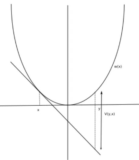
Figure 2.1: Illustration of the Bregman distance function.
2.2
Bregman Distance
In this section we give a brief overview of the Bregman distance function. These concepts will prove useful in the development of Bregman distance based algorithms in Chapter 6. In this section we will denote a general norm onRnbyk·k. The dual norm is defined and denoted ask·k∗= supkyk≤1yTx.
A convex function ω :X → R is called strongly convex with convexity parameter σ with respect to the normk·k, if it satisfies
(x−y)T(∇ω(x)− ∇ω(y))≥σkx−yk2 ∀x, y∈X◦,
where X◦ denotes the relative interior of the set X. Given a strongly convex function ω we can define the Bregman distance generating function or theprox-function V :X×X◦ →R+ induced by ω as
V(y, x) =ω(y)−
ω(x) +∇ω(x)T(y−x). (2.2.1)
The Figure 2.1 shows a graphical representation of the Bregman distance function. Note that the order of the variables as we defineV(y, x) is different from that of [26]. The following property of the Bregman distance are easy to establish and can be found in [26, 27]. Let the Bregman distance function V(·,·) be generated by a strongly convex function ω with convexity parameterσ. Then,
V(x, y) is nonnegative and for everyx∈X◦ the functionV(·, x) is strongly convex with parameter σ.
The distance functionV(y, x) can be used to define a nonlinear projection operator, also known as theprox-operator [26] as follows:
Px(y) = argminz∈X
yT(z−x) +V(z, x) . (2.2.2)
Let us consider the following convex optimization problem: minx∈X f(x), wheref(x) is a convex function and X is a convex set with nonempty interior. Let ω(x) be a strongly convex function defined onXandV(y, x) be the Bregman distance generated byω(x). Then, the Bregman distance based algorithm for this problem is given as
xk+1=Pxk(γkdk), (2.2.3)
where Px(y) is the prox-operator, dk is a subgradient of the convex function f(x) at xk and γk is the step size. The convergence of this algorithm is studied in [26], when dk is replaced by an unbiased estimate of the gradient. In the special case when the function ω(x) = 12kxk22, the Bregman function becomesV(y, x) = 12kx−yk2, and in this case the algorithm (2.2.3) reduces to the well known subgradient descent algorithm [28]
xk+1=PX[xk−γkdk], (2.2.4)
where PX is the orthogonal projection operator on the set X. Thus, Bregman distance based algorithm can be thought of as a generalization of the orthogonal projection algorithm. An in-teresting algorithm case is when the constraint set X is the probability simplex. In this case, we can equip the space with k·k1 norm, with k·k∗ = k·k∞, and choose ω as the entropy function w(x) = Pn
i=1xilogxi. This results in the Bregman function V(x, z) = Pni=1zilogzxii, and the prox-mapping takes the following form:
[P (y)] = xie
−yi
Thus, the algorithm (2.2.3) can be written as [xk+1]i= [xk]ie−γk[dk]i Pn r=1[xk]re−γk[dk]r , i= 1, . . . , n.
2.3
Basic Results
Now, we state a couple of useful standard results. The following lemma from [11] gives some relations regarding the projection operator on a convex set, where the norm k·k is the standard Euclidean norm.
Lemma 2.3.1. [11] LetX be a nonempty closed convex set inRn. Then, we have for allx, y∈X,
1. (PX[x]−x)T(x−y)≤ − kPX[x]−xk2.
2. kPX[x]−yk2 ≤ kx−yk2− kPX[x]−xk2.
3. kPX[x]−PX[y]k ≤ kx−yk.
The following known theorem, which is a generalization of the supermartingale convergence theorem will be instrumental in proving our results. The theorem is also known as the Robbins-Siegmund convergence result.
Theorem 2.3.2. ( [29], page 50) Let{Xt},{Yt},{Zt} and{gt} be sequences of random variables and let Ft, t= 0,1,2, . . . ,be a filtration such that Ft⊂Ft+1 for t≥0. Suppose that:
1. The random variables Yt, Xt, Zt and gt are nonnegative, and are adapted to the filtrationFt.
2. For each t, we have almost surely
E[Yt+1|Ft]≤(1 +gt)Yt−Xt+Zt. (2.3.1)
3. There holds P∞
t=0Zt<∞ and P∞t=0gt<∞ almost surely.
Then, almost surely, we haveP∞
t=0Xt<∞ and the sequenceYt converges to a nonnegative random
Chapter 3
Consensus Based Algorithm for
Convex Feasibility Problems
In this chapter we are concerned with the following problem. Given closed and convex setsXi ⊆Rn, i= 1, . . . , m, we need to find a point x ∈ ∩m
i=1Xi. This is a classic problem and arises in various areas of science and engineering including distributed machine learning [20], low-order control design [30] and image restoration [31] among others. A simple example of this problem arises in checking the feasibility of a given set of convex constraints in an optimization problem. In this case the constraint sets have the representation
Xi ={x∈Rn|gi(x)≤0}
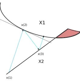
wheregi(x) is a convex function. This is a well studied problem and several algorithms have been proposed for this task. One of the most widely used algorithms is the method of successive orthog-onal projection (SOP) of Gubin, Polyak and Raik [32], also known as the method of projections onto convex sets (POCS) in the literature on image recovery [33]. There are several other vari-ants proposed for this algorithm. A comprehensive treatment can be found in the book [27]. A major drawback of the SOP algorithm is the fact that it is sequential in nature. Recently the au-thors in [11] proposed a distributed algorithm which is more amenable to be employed in a sensor network.
The main contributions in this chapter are two fold. First we propose an algorithm based on the algorithm proposed in [11] which can handle the presence of noise in the communication channel. We provide a complete analysis showing almost sure convergence of the iterates. Second we show that when the constraint sets are hyperplanes, we can explicitly characterize the convergent points of the algorithm in [11]. This result proves to be crucial in our later work on distributed machine
x(1) x(2)
x(3)
X1
X2
Figure 3.1: Illustration of the successive orthogonal projection method
The rest of the chapter is organized as follows. In Section 3.1, we provide a brief description of the SOP method along with its parallel variant. Then in Section 3.2 we formally state our problem of interest and the various assumptions. In Section 3.3 we state some preliminary results and derive our main convergence result in Section 3.4. Finally, we consider the special case of subspace constraints in Section 3.5 and provide the conclusion in Section 3.6. The results in this Chapter excluding the result in Section 3.5 is based on the results provided in [34].
3.1
Successive Orthogonal Projection
Given the closed and convex constraint sets Xi ∈Rn for i={1, . . . , m} the successive orthogonal projection method proceeds by projecting iteratively on the constraint sets. A control sequence is the order in which the constraint sets are chosen. The control sequence can be described as a mappingν :N→ {1, . . . , m}. Then the iterations of SOP proceed as follows
xk+1 =xk+γ(PXν(k)[xk]−xk), (3.1.1)
whereγ is a relaxation parameter. Forγ <1, the method is said to be under-relaxed and forγ >1, it is said to be over-relaxed [35]. Of special interest is the case when γ = 1. Convergence of the above algorithm has been studied for the general case when the sets Xi are subsets of a Hilbert space. A detailed review is provided in [35]. A drawback of the SOP algorithm is the fact that it
is sequential in nature. Some parallel algorithms have been suggested as an extension to the SOP algorithm. An algorithm suggested by Cimmino simultaneously projects on all the convex sets. Algorithmically this proceeds as
xk+1=xk+γ m X i=1 wiPXi[xk]−xk ! , (3.1.2)
where wi > 0 are weight vectors such that Pmi=1wi = 1. However, a drawback of the Cimmino algorithm is the fact that it requires a centralized hub with which all the processors need to communicate.
Next we discuss a multiprojection algorithm [27] which has an interesting interpretation in the product space and is relevant to our discussion later.
3.1.1 The Multiprojection Algorithm
Let us define the product space V =Rmn = Rn× · · · ×Rn. Given vectors x = (x1, . . . , xm) and y= (y1, . . . , ym) inV, the inner product induced onV is given ashx,yi=
Pm
i=1hxi, yii. Next, let us define in V the product set X =X1×. . . ,×Xm =Qmi=1Xi. Also, let us define the consensus subspace as ∆ ={x∈V|x= (x, . . . , x), x∈Rn}. Then the sets {X
i} have nonempty intersection if and only if the setX∩∆ is non-empty. The SOP algorithm when applied to the product space can be written as
xk+1 =PX[P∆[xk]]. On, expanding component-wise the above expression we get
xik+1 =PXi " 1 m m X i=1 xik # , (3.1.3)
where we have used the fact that in a Euclidean space with l2 norm, given a vector x ∈ V,
the projection operation is given by P∆[x] = m1 (Pmi=1xi, . . . ,Pmi=1xi). Clearly this algorithm parallelizes the PXi[·] operation. However, the operation P∆[·], either requires a central hub or a
1
m
Pm
i=1xik to a local averaging of the form
P
j∈Ni(k)wj(k)xjk, whereNi(k) is a local neighborhood of the nodei.
In the next section we formally introduce the problem setup under consideration and our proposed algorithm.
3.2
Problem Formulation
We consider a setup where we are given a set of m agents, which can be viewed as the node set V ={1, . . . , m}. We use terms node and agent interchangeably. At each timek, the communication pattern among the agents is represented by a time varying directed graph G(k). At each instant, each node receives information from a subset of nodes and, also, broadcasts its information to a subset of nodes. The subset of nodes from which a node receives information at any instant are termed as the neighboring nodes of the node at that instant. Such information exchanges are characterized by the edge set E(k) of the graph. For the scope of this paper we deal with synchronous algorithms. This implies that agents’ local clocks are synchronized and time proceeds in discrete steps k = 0,1, . . .. Let us associate with each agent i, a constraint set Xi. Each local constraint set is private and local information to node i. The objective of the network is to cooperatively solve the following optimization problem:
minimize Pm
i=1kx−PXi[x]k 2
subject to x∈Rn. (3.2.1)
When the intersection X=∩m
i=1Xi is nonempty then, a solution to the above problem is given by any vector x which lies in the constraint set X. Clearly, in this case the objective function value is zero, which is also the optimal value. Let us denote agent i0sestimate of the solution at time k by the variable xik. Since, agent ihas information only regarding his constraint set, it is desirable to require that the local estimates satisfy the constraint xik ∈ Xi, for all i and all times k. An algorithm is said to solve the problem if it generates agent estimates xik ∈ Xi that converge to a common value x∗, and x∗ satisfies the constraintx∗∈X.
a problem of constrained consensus. In this formulation the network tries to achieve consensus on the local variables xik, while satisfying the local feasibility constraint xik ∈Xi. Clearly these two viewpoint are equivalent. A distributed algorithm for this problem was proposed in [11]. In the algorithm agent ilocal variablesxik evolves as follows:
xik+1=PXi m X j=1 aij(k+ 1)xjk ,
where aij(k+ 1) denotes the weight assigned by node i to the estimate coming from node j. The problem of achieving consensus is a widely researched problem in it’s own right [1–3]. The algorithms for reaching consensus have proven useful in a wide variety of contexts from formation control [3], distributed parameter estimation [12], [13], load balancing [36], to synchronization of Kuramoto oscillators [15]. Consensus over noisy links in the lack of constraint sets has been studied in [37], [38] and [13] among others. A crucial assumption needed in the analysis in [11] was the requirement that if agent i receives data from agent j then aij(k) ≥ η > 0. We are interested in the case when the communication links are noisy and hence nodeihas access to a noise corrupted value of its neighbor’s local estimate. In this case it is detrimental to impose the requirement that aij(k)≥η since we need to asymptotically damp the impact of noise. To this effect we propose the following distributed algorithm for the problem:
xik+1=PXi " xik−αk+1 X j∈Ni(k) rij,k+1[xik−(x j k+ξij,k+1)] # .
Hereαk+1>0 is a step size,rij,k+1 is a weighting parameter,ξij,k+1 is a random variable denoting
the additive noise in communication, andNi(k) denotes the set of agents communicating with agent i at instancek. Let us definerii(k+ 1) = −Pj∈Ni(k)rij,k+1, and ξi,k+1 =
P
j∈Ni(k)rij,k+1ξij,k+1.
Then, the algorithm can be rewritten as
xik+1=PXi " xik+αk+1 m X j=1 rij,k+1xjk+αk+1ξi,k+1 # . (3.2.2)
The matrixR , whereR =r , is thus a weighted graph Laplacian and it satisfiesPm
3.2.1 Model Assumptions
In this section we state our various assumptions which are useful in deriving our convergence result. Assumption 1.
1. (Bi-directional communication) We assume that the communication is bi-directional; i.e if at any instantk,rij,k>0 then rji,k >0.
2. (Symmetric weights) The neighboring agents use symmetric weights, i.e., rij,k=rji,k.
3. (Connectedness) We assume that the graph G(k) is connected at every instance, though it is free to be time varying.
4. We assume that if rij,k6= 0 at any instant, then it satisfiesη ≤rij,k ≤η0, whereη andη0 are
positive constants.
Let us denote the filtration {Fk} as the history up to timek:
Fk={xis, ξi,s, i= 1,·, m,0≤s≤k}. (3.2.3)
We impose the following assumptions on the spatio-temporal noise process. Assumption 2.
1. The process {ξij(k)}is a martingale difference sequence, i.e., E[ξij,k+1|Fk] = 0for alli, j and k∈N.
2. At any fixed instance k, the noise on link e1 = (i1, j1) is independent of the noise on link
e2= (i2, j2) for e16=e2.
3. The noise process is uniformly bounded in the mean square sense, i.e., there is a deterministic scalar µi>0 such thatE[kξi,k+1k2|Fk]≤µ2i for allk∈N.
From Assumption 2.3, it follows that E[kξi,k+1k |Fk]≤
q
E[kξi,k+1k2|Fk]≤µi for allk∈N and all i. Let us also define µ2 =Pm
j=1µ2j. Furthermore we impose the following assumption on the step size sequence{αk}.
Assumption 3.
1. The step size in (3.2.2) is such that αk>0,
P∞
k=1αk=∞, and
P∞
3.3
Preliminary Results
In this section we provide various results which will be useful in proving our main results. Now, we establish certain relations for algorithm (3.2.2). Let
vik+1=xik+αk+1
m
X
j=1
rij,k+1xjk+αk+1ξi,k+1. (3.3.1)
Then, we have xik+1 =vik+1+eki+1,where the error term is given by eik+1 := PXi[v
i
k+1]−vik+1 =
xik+1−vki+1.
Lemma 3.3.1. When the setX =∩m
i=1Xi is nonempty, we surely have for all i∈V, k≥0, and
for all x∈X, xik+1−x 2 ≤ vik+1−x 2 − eik+1 2
Proof. By the definition of xik+1 we have
xik+1−x 2 =PXi[vik+1]−x 2 .
Now, applying Lemma 2.3.1, we get along every sample path
PXi[vki+1]−x 2 ≤ vki+1−x 2 − PXi[vik+1]−vki+1 2 =vik+1−x 2 −eik+1 2 . (3.3.2)
Let us define xk = ((x1k)T, . . . ,(xmk)T)T as the joint state vector and, similarly, ek+1, and ξk+1
be the respective stacked up versions. Define the mn×mn matrixRk+1 =Rk+1⊗In. The joint state space representation of algorithm (3.2.2) can be given as:
xk+1 = [Imn+αk+1Rk+1]xk+αk+1ξk+1+ek+1.
vectorz∈X let us denotez=z⊗1m, where 1m is them-dimensional vector of ones. Also, let us denote the conditional expectation operator Ek[·] =E[·|Fk]. Since we assume that the communi-cation graph is connected at every instant (cf. Assumption 1.3), there exists a spanning treeS(k) such that the edge (i, j) belongs to the tree if and only ifrij,k+1 > η.
Lemma 3.3.2. Let Assumptions 1 and 2 hold. Also, assume that the setX=∩m
j=1Xj is nonempty.
Then, the following relation holds for any z∈X:
Ek[kxk+1−zk2]≤H(k+ 1)kxk−zk2+α2k+1µ2−2ηαk+1 X S(k) x i k−x j k 2 , where P S(k) x i k−x j k 2
denotes summing the terms
x i k−x j k 2
over all edges arising in the spanning tree S(k).
Proof. Note that from Lemma 3.3.1 we have
Ek[kxk+1−zk2]≤Ek[kvk−zk2]−Ek[kek+1k2], (3.3.3)
wherevk= [Imn+αk+1Rk+1]xk+αk+1ξk+1. Hence,
Ek[kvk−zk2] =k[Imn+αk+1Rk+1]xk−zk2+α2k+1Ek[kξk+1k2]
+ 2αk+1([Imn+αk+1Rk+1]xk−z)TEk[ξk+1].
By our Assumption 2.1 Ek[ξk+1] = 0, so that
Ek[kvk−zk2] =k[Imn+αk+1Rk+1]xk−zk2+α2k+1Ek[kξk+1k2].
Since Rk+1 is symmetric and has zero-row sums, we have
k[Imn+αk+1Rk+1]xk−zk2= [xk−z]T[Imn+αk+1Rk+1]T[Imn+αk+1Rk+1] [xk−z]
We also have
[xk−z]T RTk+1Rk+1[xk−z]≤σ2m(Rk+1)kxk−zk2,
whereσm(Rk+1) is the maximum singular value of the matrixRk+1. SinceRk+1 =Rk+1⊗In, we have σm(Rk+1) =σm(Rk+1). Hence,
[xk−z]T[Imn+α2k+1RTk+1Rk+1][xk−z]≤H(k+ 1)kxk−zk2,
withH(k+ 1) = 1 +α2
k+1σ2m(Rk+1).
Now, consider the term [xk−z]TRk+1[xk−z] in (3.3.4). SinceRk+1 has row sum zero andRk+1
is symmetric, we haveRk+1z= 0 and zTRk+1 = 0. Thus,
[xk−z]TRk+1[xk−z] =xTkRk+1xk.
By definition Rk+1 = Rk+1⊗Im, where rij,k+1 =rij,k+1 and Rii,k+1 =−Pmj=1,j6=irij,k+1. Thus,
we see that xTkRk+1xk=− m X i=1 (xik)T m X j=1,j6=i rij,k+1(xik−x j k). Since, the matrix Rk+1 is symmetric we have
− m X i=1 xTi (k) m X j=1,j6=i rij,k+1(xik−x j k) =− X i<j rij,k+1 x i k−x j k 2 ≤ −ηX S(k) x i k−x j k 2 , whereP S(k) x i k−x j k 2
denotes summing the terms
x i k−x j k 2
over all edges arising in the span-ning tree. Using the preceding relation and the bound Ek[kξk+1k2]≤µ2 we arrive at
Ek[kvk−zk2]≤H(k+ 1)kxk−zk2+α2k+1µ2−2αk+1η X S(k) x i k−x j k 2
By substituting back in Eq. (3.3.3) we get
Ek[kxk+1−zk2]≤H(k+ 1)kxk−zk2+α2k+1µ2−2αk+1η X x i k−x j k 2 −Ek[ke(k+ 1)k2].
Neglecting the error term we have the desired result.
3.4
Convergence Result
In this section we state and prove our main convergence result for the algorithm (3.2.2). Theorem 3.4.1. Assume that X =∩m
j=1Xj is nonempty, and let Assumptions 1 and 2 hold. Let
the step size sequence{αk} in algorithm (3.2.2) satisfy Assumption 3. Then, there exists a random
variablex∗ taking values in the setXsuch that almost surelylimk→∞
xik−x∗
= 0for all agentsi.
Proof. First, we consider the termH(k+1) = 1+α2k+1σm2(Rk+1) in Lemma 3.3.2. The entries of the
matrixRk+1 are uniformly bounded, implyingσ2m(Rk+1)≤C for some scalarC and all k. By our
assumption on the step size, we haveP∞
k=1αk2 <∞. Since all the terms appearing in Lemma 3.3.2 are nonnegative, we can apply the result of Robbins-Siegmund (Theorem 2.3.2) to deduce that, with probability one, kxk−zk2 converges for any z∈X and
∞ X k=1 αk+1 X S(k) x i k−x j k 2 <∞. (3.4.1) By P∞
k=1αk =∞, relation (3.4.1) implies that there is a subsequence such that lim k→∞ X S(nk) kxi nk−x j nk|| 2 = 0.
Now, since the number of spanning trees on a finite graph is finite, there exists a spanning tree S which appears infinitely often in the sequence {S(nk)}. Let us pick a further subsequence such that S(n1k) = S, then we have along this subsequence limk→∞PS
x i n1 k −xjn1 k 2 = 0 for all i and j. The spanning tree S is in the connected graph, so the preceding relation yields limk→∞ x i n1 k −xjn1 k 2
= 0 for alli, j. Now sincekxk−zk2 converges almost surely for any z∈X, the subsequence {xn1
k} is bounded almost surely. Again, we can extract a convergent subsequence
xn2
k such that limk→∞
x i n2 k −x∗i
= 0 almost surely for some random vector x
∗
i for all i. Since lim k→∞ x i n2 k −xjn2 k = 0
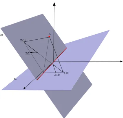
Figure 3.2: Illustration of Distributed Algorithm whenXi are subspaces
almost surely for all i, j, it follows that x∗i = xj∗ = x∗ almost surely for all i, j. The sets Xi are closed, so that x∗ ∈ Xi almost surely for all i, which in turn implies that x∗ ∈X almost surely. Therefore, limk→∞kxn2
k−x
∗k2 = 0 almost surely. But, we know that lim
k→∞kxk−zk2 converges almost surely for all z ∈ X. Hence, by looking at the sample paths, we can conclude that the limit of any subsequence is also the sequential limit, implying that limk→∞kxk−x∗k= 0 almost surely.
3.5
Subspace Constraints
In this section we provide a unique result which holds when the constraint sets Xi are subspaces. It was shown by Von Neumann [39] that the infinite product of the operatorPX2PX1, whenX1 and X2 are subspaces in a Hilbert space, converges to the operator PX1∩X2, i.e limk→∞[PX2PX1]
k = PX1∩X2. This result was extended by Halperin [40] to a finite number of subspaces. We essentially i
algorithm has the property that asymptotically the iterations converge to the projection ofx0 on
the intersection of the subspaces X.
In this section we restrict ourself to the noiseless case. In the noiseless case our algorithm is same as the one provided in [11]
xik+1=PXi " m X j=1 wij,k+1xjk # . (3.5.1)
In this case, we assume that the underlying space X ⊆ H, is a finite dimensional Hilbert space. Hence, the projection operation PXi is now understood in terms of minimizing the Hilbert space
norm k·kH on H. The constraint sets Xi have the following kernel representation in terms of a linear operatorAi:H → R(Ai):
Xi ={x∈ H:Aix= 0}.
Equivalently Xi could be represented as
Xi ={x∈ H:hzij, xiH= 0, zij ∈ H, j= 1, . . . , ki}.
In this case the operatorAi can be constructed as
Aix= hzi1, xiH .. . hziki, xiH .
Let us denote the kernel of the operatorAi asN(Ai). Let us define the joint operator
A= A1 .. . Am .
Then it is clear that X = N(A) = ∩m
j=1Xj = {x ∈ H : Ax = 0}. Let us denote the projection operator on the kernel of Ai asHi. Let us denoteA∗i as the adjoint operator ofAi, then, it can be
checked that
Hi =I−A†iAi,
whereA†i =A∗i(A∗iAi)−1 is the pseudoinverse operator. Then our algorithm can be written as
xik+1 =Hi[ m
X
j=1
wij,k+1xjk].
We now have the following result.
Theorem 3.5.1. Let us assume that the constraint sets Xi are subspaces. Given any pointx0∈ H,
let us initialize xi1 = PXi[x0]. Then the iterations of the algorithm 3.5.1 converge to a common
pointx∗∈X, such thatx∗=PX[x0], where X=∩mi=1Xi.
Proof. We know from our analysis earlier that each of the iterates xik converges to the same point x∗ in X. We want to show that the point x∗ is the projection of x0 on X. In other words we
want to show thatx∗−x0 ⊥ N(A) =X. Since,R(A∗)⊥ N(A), this is equivalent to showing that
x∗−x0∈ R(A∗). We will prove this by induction. First, let us notice that for alli
xi1 =Hix0= [I−A†iAi]x0,
we have xi1−x0=−Ai†Aix0. Thus, xi1−x0 ∈ R(A∗i)⊆ R(A∗). Thus we can rewrite xi1 =x0+v1i,
wherevi1 ∈ R(A∗). Now, let us assume that for alliwe can writexik=x0+vki, wherevik∈ R(A
∗).
Now, since xik+1 =Hi[Pmj=1wij,k+1xjk], it follows that
xik+1− m
X
j=1
wij,k+1xjk∈ R(A∗i)⊆ R(A
∗).
Hence,xik+1−Pm
j=1wij,k+1xjk =si(k+ 1), for an element si(k+ 1)∈ R(A
∗). Now, plugging back
from our induction step we get
xik+1− m
X
j=1
Using the fact that Pm
j=1wij,k+1 = 1, we get that
xik+1−x0 =
m
X
j=1
wij,k+1vkj +si(k+ 1).
Since vkj ∈ R(A∗), and s
i(k+ 1) ∈ R(A∗), we deduce that xik+1−x0 ∈ R(A∗). Now, denoting
vki+1 = Pm
j=1wij,k+1vj(k) +si(k+ 1), we can rewrite xik+1 = x0 +vki+1. From the principle of
mathematical induction we can deduce that xik −x0 ∈ R(A∗). Thus, since R(A∗) is a closed
subspace we havex∗−x0 ∈ R(A∗).
3.6
Conclusion
In this Chapter we provided a distributed algorithm for the convex feasibility problem. The al-gorithm can be applied over a time varying network with stochastic noise in the communication links. The algorithm resembles a stochastic approximation scheme by utilizing a diminishing square summable step size sequence to mitigate the effect of communication noise. For the noiseless case we characterized the convergent point of the algorithm when the constraint sets are subspaces. In Chapter 5 we extend the proposed algorithm to the asynchronous setting. We also establish asymptotic error bounds for the case when the step size αk is chosen to be a constant.
Chapter 4
Synchronous Algorithm for
Distributed Constrained Stochastic
Optimization
In this chapter we consider the general problem of solving the distributed optimization problem when the objective function is a sum of m local convex objective functions corresponding to m agents. The objective of the agents is to cooperatively solve the following constrained optimization problem: minimize m X i=1 fi(x) subject to x∈X= m \ i=1 Xi, (4.0.1)
where each fi :Rn →R is a convex function, representing the local objective function of agent i, and each set Xi ⊆Rn is a compact and convex set, representing the local constraint set of agent i. Since the objective function is continuous and the set X is compact, we know by Weirstrass theorem that the optimal set is nonempty. Let us denote the optimal set by X∗. We assume that the local constraint set Xi and the objective function fi are known to agent i only. In this formulation the local objective functions are allowed to be of the form
fi(x) =Ez[Li(x, z)] + Ω(x),
where the expectation is over the unknown distribution of random variable z and Ω(x) is a not necessarily differentiable function of x. Such formulations naturally arise in problems related to machine learning [41, 42], which is dealt in more detail in Chapter 7. Ω(x) is a regularization term included to improve the generalization ability [43]. Recently a lot of interest in signal processing has been generated towards the use of thel1-norm as the regularization term. In many cases it has been
our algorithm which doesn’t require the objective function to be differentiable is suitable for this problem. It is well known that the stochastic optimization problems of the form above can be dealt with by using first-order stochastic gradient descent methods [44]. Such algorithms are also known as stochastic approximation algorithms. Let us denote by∂fi(x), the subdifferential offi(x). Then a centralized solution to the problem is given by the following projected subgradient algorithm.
xk+1 =PX " xk−αk m X i=1 dik # , (4.0.2)
where dik ∈∂fi(xk), and αk is a step size sequence. In [6], an incremental subgradient algorithm was proposed for this problem. This algorithm shares the sequential nature of the SOP algorithm. We now briefly discuss the algorithm.
4.1
Incremental Subgradient Algorithm
The incremental subgradient algorithm proceeds by incrementally updating the vectorxthrough a sequence ofm steps. At each step only the subgradient information corresponding to the objective function fi is used. Similar to the SOP algorithm let us define a control sequence as a mapping ν :N→ {1, . . . , m}. Then the iterations of the incremental subgradient algorithm suitable adapted to the our problem can be written as
xk+1=PXν(k)
h
xk−αkdνk(k)
i
, (4.1.1)
where dνk(k) ∈ ∂fν(k)(xk). This algorithm recovers the SOP algorithm for the case when fi(x) =
1
2kx−PXi[x]k 2
. In this casedik=xk−PXi[xk]. Substituting back in Eq (4.1.1) for the caseαk= 1
we get
xk+1 =PXν(k)[xk], (4.1.2)
which is the SOP algorithm Eq (3.1.2) forγk= 1. In its original form the incremental subgradient algorithm was designed for deterministic cyclical control sequences. This requirement was relaxed in [8], in which the authors considered the case when the control sequence could be a sample path of an evolving Markov chain.
4.2
The Stochastic Optimization Problem
In this section we briefly talk about how the stochastic optimization problem when the objective functions are of the form fi(x) = Ez[Li(x, z)], can be incorporated in our framework. Here z is a random variable and the expectation is taken with respect to the unknown distribution of the random variable. Thus the function fi(x) is not known to agent i. The agent i however has access to samples ofz. Let∇xf(x) denote a subgradient of the objective functionf(x) then under some broad assumptions it can be shown that ∇xfi(x) = E[∇xLi(x, z)]. Hence, we can write ∇xfi(x) = ∇xLi(x, z) + [E[∇xLi(x, z)]− ∇xLi(x, z)]. Denoting i := E[∇xLi(x, z)]− ∇xLi(x, z), we can see that it is a martingale difference sequence,
E[i|Fk] = 0.
Thus, we can see that the stochastic optimization problem can be fit in the gradient descent framework by including an error term which satisfies the criterion of being a martingale difference sequence.
The rest of this Chapter is organized as follows. In Section 4.3 we discuss various example which motivate the specific problem structure we consider in (4.0.1). In Section 4.4 we state our main algorithm for the problem under consideration and provide our assumptions. In Section 4.5 we state and prove some preliminary results which are useful in deriving our convergence result in Section 4.6. Finally in Section 4.7 we provide a brief conclusion. This Chapter is based on the results provided in [34].
4.3
Distributed Optimization Problems Arising In Networks
In this section we discuss several problems which arise in sensor networks and emphasize that the common theme among these problems is the fact that they can be cast as distributed optimization problems.4.3.1 Consensus and Robust Estimation
The problem of achieving consensus in a sensor network has seen tremendous amount of research in recent times. This is fueled by the fact that many problems arising in distributed control and estimation can be approached by using this machinery. The basic problem of consensus is the following. Let us assume that each sensor makes an observation at time 0 denoted as zi(0). The objective of the network is for each sensor to compute the average ¯z= m1z0i of the observations. It can be easily seen that this is equivalent to solving the following optimization problem
minimize x 1 m m X i=1 z0i −x 2 .
The optimal solution to the above problem is given byx∗= m1 Pm
i=1z0i. A variant of the consensus
problem was posed in [16], which the authors termed as the robust estimation problem. In their framework the sensors have the observations {zi
t} for t = (0, . . . , T). The objective is to again compute the average value ¯z = mT1 PT
t=0
Pm
i=1zti. However, unlike the quadratic loss function which is used in the consensus problem they proposed the Huber loss function, which is defined as
ρ(z, x) = kz−xk2/2 kz−xk ≤γ γkz−xk −γ2/2 kz−xk> γ,
where γ is a fixed parameter. The objective of the sensor network is to solve the following opti-mization problem minimize x 1 mT m X i=1 T X t=0 ρ(zti, x).
The choice of the Huber loss function makes the network less susceptible to outliers in the data collection process as less weight is given to data which deviates more than the chosen parameterγ.
4.3.2 Constrained Estimation
Now, let us consider the case of estimation of a parameter in a sensor network of heterogeneous sensors. In this formulation the assumption of Gaussian noise is relaxed to include noise with
bounded support. In the linear case the ith sensor observation is modeled as follows.
zi(t) =θTxi(t) +wi(k) for t= 0, . . . , T
where the noise wi(t) has the following truncated Gaussian distribution.
pwi(w) = 1 K√2πσ2 i exp(−w2 2σ2 i ) if|w| ≤bi 0 otherwise,
where K is the normalization constant. Here the truncated Gaussian noise models the sensor characteristics and are assumed to be different for different sensors. It is assumed that the initial
a priori information about the parameter is modeled as a GaussianN(µ0, P0) distribution. In this
case it can be shown that the maximum posteriori estimate (MAP) is given by the solution of the following optimization problem
minimize θ m X i=1 T X t=1 1 2σ2i|zi(t)−θ Tx i(t)|2+ 1 2(θ−µ0) TP−1 0 (θ−µ0) subject to |zi(t)−θTxi(t)| ≤bi ∀ t= 1, . . . , T ∀i= 1, . . . , m
This is an optimization problem of the form
minimize θ m X i=1 fi(θ) subject to θ∈ m \ i=1 Xi whereXi:={θ:|yik−θiTxik| ≤bi ∀ k= 1, . . . , N}.
This formulation illustrates the need to come up with distributed solutions schemes for the parameter estimation problem when different sensors have a-priori information about the parameter lying in different convex constraint sets.
4.3.3 Network Utility Maximization in a Wireless Network
The problem of fair allocation of resources has been thoroughly studied in the area of microeco-nomics [21]. Recent interest in the resource allocation problem has arisen in the context of utility maximization in communication networks [24]. One of the most important characteristics of the network utility maximization problem is the fact that the objective function to be minimized has a separable form. Under this structure various primal or dual decomposition methods can be applied to make the problem amenable to a distributed solution [45]. Various problems arising in network utility maximization (NUM) can be formulated as one of maximizing
maximize x m X j=1 Uj(x1, . . . , xm) x∈X.
An illustrative example is provided in [17], where it is shown that the problem of distributed power control in a wireless network can be formulated as
min x m X i=1 log σi2h −2 i,ie −xi+X j6=i h−i,i2h2j,iexj−xi +V(exi) subject to x∈X,
whereV is a convex and increasing function. Clearly this problem fits in our framework. We show in Chapter 6 that a variant of the above sum utility maximization problem which maximizes the minimum utility allocated can also made to fit in our framework after a suitable transformation.
4.3.4 Distributed Model Predictive Control
Model predictive control also known as receding horizon control is a widely popular technique to solve infinite horizon optimal control problems. It is typically employed in situations when the presence of constraints renders the dynamic programming solution of the infinite horizon optimal control problem infeasible. It solves the infinite horizon problem in a batch framework , where in each batch a finite time horizon nonlinear programming problem is solved. For a detailed treatment
refer to [46]. Distributed model predictive control arises naturally in many situations when there are multiple plants and controllers connected over a network. A survey of different architectures employed for distributed MPC can be found in [47] and the problems associated with coordinating multiple MPC based controllers can be found in [48]. Recently this approach has been applied to the problem of coordination of multiple unmanned air vehicles [49]. The difficulty in solving the distributed MPC problem stems from the coupling, which arises between different agents through the cost function, dynamics or constraints. We present the distributed MPC formulation from [50], which fits our framework.
There areminterconnected subsystems, where for each subsystemithere is associated a local state xi ∈ Rni, and a control vector ui ∈ Rpi. The coupling among the subsystems is captured by the graphG= (V, E). The state equation for theith subsystem is given as
xik+1=Aixik+
X
j∈Ni
Bijuj(k),
whereNi is the set of neighbors of nodei. The MPC problem is to solve the following optimization problem min u Pm i=1Φi =Pmi=1 PT k=1 1 2[(x i k)0Qixik+ui(k−1)0Riui(k−1)] subject to xi k+1 =Aixik+ P j∈NiBijuj(k) x i k∈ Xi,ui(k)∈ Ui ∀i,
where Ui is the local closed, convex and compact constraint set on the control action of system i. Let us denote ¯ xi= xi1 .. . xiT and u¯i= ui(0) .. . ui(T−1) .
Then, it can be verified that we can write
¯ xi= ¯Aixi(0) + X j∈Ni ¯ Biju¯i, (4.3.1)
where ¯Ai and ¯Bij can be easily derived. Since the equation 4.3.1 is an affine function of ¯ui, constraint xik ∈ Xi can now be translated into a convex constraint on ¯ui, as ¯ui ∈ Ui0. Thus, the variable ¯ui ∈ Ui∩Ui0:=Ui. Note thatUiis the constraint set in the product space. The optimization problem can similarly be written as
min u m X i=1 Φi Φi= 12xi(0)0A¯0iQ¯iA¯0ixi(0) +Pj∈Nixi(0) ¯A 0 iQ¯iB¯iiu¯i+12Pj∈I(i) P k∈Niu¯ 0 iB¯ijQ¯iB¯iju¯j+12u¯iR¯iu¯i subject to u¯i∈Ui.
4.4
Main Algorithm
We propose the following subgradient algorithm:
xik+1 =PXi " xik−αk+1 X j∈Ni(k) rij,k+1[xik−(x j k+ξij,k+1)]−γk+1[dik+1+ik+1] # .
Here, the vector dik is a subgradient of the local objective function fi and ik+1 is the error in the
evaluation of the subgradient of fi(x) at x =vki+1, where vik+1 is given by (3.3.1). The step size γk+1 >0 is used to attenuate the subgradient error. Proceeding similarly to the consensus part let
us rewrite this as follows.
vki+1=xik+αk+1 m X j=1 rij,k+1xjk+αk+1ξi,k+1 xik+1 =PXi vki+1−γk+1[dik+1+ik+1] . (4.4.1)
We denote the noisy subgradient by ˜dik = dik+ik. There are several interesting aspects of the algorithm (4.4.1). The algorithm relies on the consensus enforcing term in the calculation ofvki+1to ensure that the agents estimates converge to a common optimal point. The idea of using projection on local constraint sets PXi[·] is taken from the SOP algorithms. Furthermore the algorithm
noise respectively. Our analysis reveals an interesting interplay between these step sizes for which almost convergence can be proven for the algorithm. The use of diminishing step size sequences to handle subgradient noise arises in the stochastic approximation literature. To sum up, the proposed algorithm uses aspects of consensus algorithms, SOP algorithms and the stochastic approximation technique to provide a distributed algorithm for the optimization problem (4.0.1).
We next state the various assumptions needed to derive our convergence result.
4.4.1 Assumptions
Let∂fi(x) denote the set of subgradients of the objective functionfi(x). We impose the following assumptions on the subgradients and the constraint sets.
Assumption 4.
1. The subgradient errors ik when conditioned on the point of evaluation of the subgradient dik
are mean zero, i.e., E[ik|vki] = 0 for alli andk≥0.
2. The subgradient errors further satisfy the bound E[ik
2
|vi
k]≤ν2 for alli and k≥0.
3. The local constraint sets Xi are compact and convex.
4. The intersection set X has a nonempty interior, i.e., there exists a pointz¯∈X such that the ball Bδ :={x∈X :kx−zk ≤¯ δ} ⊂X.
In addition to the above assumptions on the model, we use the following assumptions on the step sizesαk and γk.
Assumption 5.
1. (non-summability) The step sizes satisfy P∞
k=1αk=∞ and P∞ k=1γk=∞. 2. (square summability) P∞ k=1α2k<∞ and P∞ k=1γk2<∞. 3. P∞ k=1αkγk <∞ and P∞k=1 γ2 k αk <∞. 4. P∞ k=1min{αk, γk}=∞.
The Assumptions 5.1 and 5.2 are standard in the stochastic approximation literature. The square summability is needed to damp out the noise terms. In addition to these conditions, our analysis relies on Assumptions 5.3 and 5.4 on the cross terms involving the step sizes. To verify that the set of step sizes satisfying these conditions is non empty, we can assume that the step sizes are of the form αk = k1θ1 and γk =
1
kθ2. Then conditions 5.1 and 5.2 imply that 1/2< θ1, θ2 ≤1. It is clear
that in this caseP∞
k=1αkγk<∞. The conditionP∞k=1 γ2 k αk <∞implies thatθ2 > 1+θ1 2 . Also, since
whenθ2> θ1, we have min(αk, γk) =γk; and in this case Assumption 5.4 holds by Assumption 5.1.
4.5
Preliminary Results
In this section we provide some results which will be useful in deriving our main result. The first result provides a way to bound an error term of the formxik−PXi[xik]
. The bound is established
by using some of the techniques in [32] for the alternating projection method.
Lemma 4.5.1. Let Assumptions 4.3 and 4.4 hold, and let xi ∈Xi be variables belonging to local
constraint sets Xi. Then, we have the following bound:
kxi−PX[xi]k ≤ B δ m X j=1 kxi−xjk for all i,
where B is a uniform upper bound on the norms of the vectors in the sets Xi and δ is the radius
from Assumption 4.4.
Proof. Let ibe arbitrary. Defineλi=Pmj=1kxi−PXj[xi]k and the variablesi as follows:
si = λi λi+δ ¯ z+ δ λi+δ xi,
where ¯z is the interior point of the set X from Assumption 4.4. Then, we can write
si = λi λi+δ ¯ z+ δ λi xi−PXj[xi] + δi λi+δ PXj[xi].
From definition of λi, it is clear that
xi−PXj[xi]
≤λi for anyj, implying by the interior point
assumption that the vector ¯z+ λδ
i xi−PXj[xi]
j. Since the vector si is a convex combination of two vectors in the set Xj, by the convexity assumption on the set Xj, we have that si ∈ Xj for any j. Therefore, we have si ∈X. Now, we can see that
kxi−sik ≤ λi λi+δ kxi−zk ≤¯ kxi−zk¯ δ m X j=1 xi−PXj[xi]
By our assumption the sets Xi are compact, so kxi−zk ≤¯ B for B > 0. Since xj ∈Xj, by the properties of the projection operator it follows xi−PXj[xi]
≤ kxi−xjk. Thus, kxi−PX[xi]k ≤ kxi−sik ≤ B δ m X j=1 kxi−xjk.
Let us define sk = m1 Pmj=1PX[xjk], which belongs to the set X since X is closed and convex. The following lemma is crucial in proving our convergence result in the next section.
Lemma 4.5.2. Let Assumptions 1, 2 and 4 hold. Then, for the algorithm proposed in Eq. (4.4.1)
the following relation holds for any z∗ in the optimal set X∗,
Ek[kxk−z∗k2]≤H(k+ 1)kxk−z∗k2+α2k+1µ2−αk+1η X S(k) x i k−x j k 2 +m(ν+C)2γk2+1+K 2γ2 k+1 ηαk+1 −2γk+1[f(sk)−f(z∗)] + 2Cγk+1αk+1 m X i=1 m X j=1 rij,k+1xjk ,
where C is a uniform bound on subgradient norms of fi over the sets Xi, K =C(m−1)(mBδ+δ)
and f(x) =Pm
i=1fi(x).
Proof. By definition we have xik+1 =PXi[v
i
k+1−γk+1d˜ik+1]. From the contraction property of the
projection operator we see that for any z∗ ∈X∗ ⊆X,
xik+1−z∗ 2 ≤ v i k+1−z∗−γk+1d˜ik+1 2 =vki+1−z∗ 2 +γk2+1 ˜ dik+1 2 −2γk+1( ˜dik+1)T(vik+1−z ∗ ). (4.5.1)
Taking conditional expectation, we obtain for any z∗ ∈X∗, Ek[xik+1−z∗ 2 ]≤Ek[vik+1−z∗ 2 ] + 2γk2+1Ek[ ˜ dik+1 2 ] −2γk+1Ek[(dik+1)T(vki+1−z ∗ )]−2γk+1Ek[(ik+1)T(vik+1−z ∗ )].
Since, Ek[(ik+1)T(vik+1−z∗)] = Ek[(vik+1−z∗)TE[ik+1|vik+1]] and E[ik+1|vki+1] = 0 and dik+1 is a
subgradient offi atvik+1, we have Ek[xik+1−z∗ 2 ]�