Denoising Source Separation
Jaakko S¨arel¨a [email protected]
Neural Networks Research Centre Helsinki University of Technology
P.O.Box 5400, FI-02015 HUT, Espoo, FINLAND
Harri Valpola [email protected]
Artificial Intelligence Laboratory University of Zurich
Andreasstrasse 15, 8050 Zurich, Switzerland
orNeural Networks Research Centre Helsinki University of Technology
P.O.Box 5400, FI-02015 HUT, Espoo, FINLAND
Editor:????
Abstract
A new algorithmic framework called denoising source separation (DSS) is introduced. The main benefit of this framework is that it allows for easy development of new source separa-tion algorithms which are optimised for specific problems. In this framework, source sep-aration algorithms are constucted around denoising procedures. The resulting algorithms can range from almost blind to highly specialised source separation algorithms. Both sim-ple linear and more comsim-plex nonlinear or adaptive denoising schemes are considered. Some existing independent component analysis algorithms are reinterpreted within DSS frame-work and new, robust blind source separation algorithms are suggested. Although DSS algorithms need not be explicitly based on objective functions, there is often an implicit objective function that is optimised. The exact relation between the denoising procedure and the objective function is derived and a useful approximation of the objective function is presented. In the experimental section, various DSS schemes are applied extensively to artificial data, to real magnetoencephalograms and to simulated CDMA mobile network signals. Finally, various extensions to the proposed DSS algorithms are considered. These include nonlinear observation mappings, hierarchical models and overcomplete, nonorthog-onal feature spaces. With these extensions, DSS appears to have relevance to many existing models of neural information processing.
Keywords: blind source separation, BSS, prior information, denoising, denoising source separation, DSS, independent component analysis, ICA, magnetoencephalograms, MEG, CDMA
1. Introduction
(BSS). Independent component analysis (ICA) (Hyv¨arinen et al., 2001b) clearly follows this tradition. This blind approach certainly has its assets, giving the algorithms a wide range of possible applications. ICA has been a valuable tool, in particular, in testing the hypotheses of the target field of research (c.f.,Vig´ario et al., 2000).
Nearly always, however, there is further information due to the experimental setup, other design specifications or cumulated knowledge due to scientific research. For example in biomedical signal analysis (c.f., Gazzaniga, 2000, Rangayyan, 2002), careful design of experimental setups provides us with presumed signal characteristics. In man-made tech-nology, such as a CDMA mobile system (c.f., Viterbi, 1995), the transmitted signals are even more restricted.
The Bayesian approach provides a sound framework for including prior information into inferences about the signals. This has been used, for instance, by Knuth (1998), Valpola and Karhunen (2002), S¨arel¨a et al. (2001). However, the algorithms are not always simple or computationally efficient. In fast point estimate algorithms, prior information has been used for denoising the results given by ICA (Vigneron et al., 2003). Additional information has also well been used to extract signals corresponding to some specific feature of the measured phenomenon (for a review of biomedical applications, see Rangayyan, 2002).
In this paper, we introduce denoising source separation (DSS), a new framework for incorporating prior knowledge into the separation process. DSS is developed by generalising the principles introduced by Valpola and Pajunen (2000). We argue that it is often easy and practical to express the available knowledge in terms of denoising.
Some previous works (c.f., Hyv¨arinen et al., 1999, Valpola and Pajunen, 2000) have acknowledged that it is possible to interpret some parts of ICA algorithms as denoising. In this paper, we show that it is actually possible to construct the source separation algorithms around the denoising methods themselves.
Denoising corresponds to procedural knowledge. This differs from most approaches to ICA where the algorithms are derived from explicit objective functions leading to declara-tive knowledge. We also derive the exact relation between the objecdeclara-tive function and the corresponding denoising. This makes it possible to mix the two types of information and also provides a new interpretation to some of the existing ICA algorithms.
Additionally, we review a method to speed up convergence and discuss the applicability of DSS for exploratory source separation when no detailed information of the sources is available.
The paper is organised as follows: In Sec. 2, we introduce the principles of denoising source separation in a linear framework and proceed to nonlinear denoising. In Sec. 3, some practical denoising functions are discussed. In Sec. 4, a useful approximation for the objective function of DSS is derived and its uses are discussed. The use of the algorithmic framework is demonstrated in Sec. 5 in experiments with artificial and real-world data. Finally, in Sec. 6, we discuss extensions to DSS framework and their connections to models of neural information processing.
2. Source separation by denoising
Consider a linear instantaneous mixing of sources:
where X= x1 x2 .. . xM
, S=
s1 s2 .. . sN . (2)
The source matrix S consists of N sources. Each individual source si consists of T
sam-ples, that is, si = [si(1) . . . si(t) . . . si(T)]. Note that in order to simplify the notation
throughout the paper, we have defined each source to be a row vector instead of the more traditional column vector. The symbol t often stands for time, but other possibilities in-clude, e.g., space. For the rest of the paper, we refer to t as time, for convenience. The observationsXconsist ofM mixtures of the sources, that is,xi = [xi(1). . . xi(t). . . xi(T)].
Usually it is assumed thatM ≥N. The linear mappingA= [a1a2 · · ·aM]T consists of the
mixing vectors ai = [ai1ai2 . . . aiN]T, and is usually called mixing matrix. In the model,
there is some Gaussian noiseν, too.
If the sources are assumed Gaussian, this is a general, linear factor analysis model with rotational invariance. There are several ways to fix the rotation,i.e., to separate the original sources, S. Some approaches assume structure for the mixing matrix. If no structure is assumed, the solution to this problem is usually called blind source separation (BSS). Note that this approach is not really blind, since one always needs some information to be able to fix the rotation. One such information is the non-Gaussianity of the sources, which leads to the recently popular ICA methods (c.f.,Hyv¨arinen et al., 2001b). Other properties may include their temporal structure as in Belouchrani et al. (1997), Ziehe and M¨uller (1998).
In this section we introduce a general framework for using denoising algorithms for source separation. We show how source separation algorithms can be constructed around methods for removing noise from the estimated sources. We first analyse the situation in linear denoising and then consider the nonlinear case.
2.1 Linear denoising
Many ICA algorithms preprocess the data by removing the mean and normalising the covariance to unit matrix, i.e., XXT/T =I. This is referred to as sphering, whitening or decorrelation and its result is that any signal obtained by projecting the sphered data on any unit vector has zero mean and unit variance. Furthermore, orthogonal projections yield uncorrelated signals. Often sphering is combined with reducing the dimension of the data by selecting a principal subspace which contains most of the energy of the original data. In ICA, the motivation for sphering is that with at most as many sources as observations, the original independent signals can be recovered by an orthogonal rotationW of the sphered signals, provided that the noiseν is negligible. If there is substantial noise present, unbiased estimate for S may not be achieved by an orthogonal W. Even in these cases, orthogonal W usually offers a good approximation. For the rest of the paper, the data X is assumed to be spherical or sphered and we mainly consider orthogonal rotationsW.
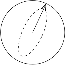
Figure 1: Sphering renders the variance of all unit projections equal and the projections can be depicted by a circle (solid line). After denoising (dashed line), the variance depends on the direction of the projection, and the signal or signals of interest can be identified by PCA. The arrow points to the direction of the first principal component.
with unit variance and, more importantly, not all projections result in the same variance. After low-pass filtering, it is therefore possible to identify the signals having higher than average proportion of low frequencies by principal component analysis (PCA).
If signals of interest are characterised as having low-frequency components, low-pass filtering can be regarded as denoising. It is thus possible to identify the following steps in the above signal separation: sphering, denoising and PCA. These are illustrated in Fig. 1.
For now we consider linear denoising. This means that denoising can be mathematically expressed as matrix multiplication. Then for denoising matrix D the denoised data Z becomes:
Z=XD. (3)
Note that D operates on each signal xi separately, i.e., denoising is defined for
one-dimensional signals. Furthermore, the denoising is performed over time, i.e., D is T ×T -matrix.
The first principal component of the denoised data Z, can be computed by the classical power method (see any elementary matrix textbook):
w+=ZZTw (4)
wnew= w+
||w+||, (5)
where wnew, a column vector, means the new estimate of the principal direction. This power method finds the maximum eigenvector1 of the covariance matrix of the denoised data. Thus its objective function is
subject to the constraint wTw = 1. Note that glin(w) is a scalar function of a vector argument.
Let us now substitute the denoising (3) into the power method (4):
w+=ZZTwT =XDDTXTw. (7)
Further, let us denote
D∗ =DDT. (8)
Then the classical power method applied to filtered data can be reformulated as follows:
s=wTX (9)
s+=sD∗ (10)
w+=Xs+T (11)
wnew= w+
||w+||, (12)
where s is used to denote the current estimate of the signal corresponding to the eigen-vector estimate w. From now on, we shall refer to this signal as source. Mathemati-cally, algorithm (9)–(12) is equivalent to the classical power method applied to the filtered data (3)–(5). In the classical version, the denoising D was applied to the whole data, but in Eq. (10) the denoising D∗ is applied to the current source estimate s, instead. Equa-tions (11) and (12) compute the weight vector which yields a new source which is closest to the denoiseds+ in the least-mean-squares (LMS) sense. We call Eqs. (9)–(12) thelinear DSS algorithm. The corresponding objective function, starting from Eq. (6), can be written as
glin(s) =wTZZTw=sD∗sT, (13) In order to study further the relation between D∗ and D, let us now assume that D∗ is given and try to find a corresponding D that satisfies Eq. (8). Since DDT is always symmetric, a necessary condition for the existence of a correspondingDis symmetry ofD∗. In this case it means symmetry in time since D∗ is a T ×T matrix. Symmetric matrices have an eigenvalue decomposition
D∗ =VΛ∗VT, (14)
whereΛ∗ is diagonal andVis orthonormal2. SinceD=VΛ∗1/2 satisfies Eq. (8), symmetry of D∗ is both a necessary and sufficient condition for the existence of a correspondingD. Power method applied to the denoised dataZ always converges (assuming that the largest eigenvalue is not degenerate). The above analysis shows that the same holds for linear DSS provided that denoising is symmetric in time.
The eigenvalue decomposition (14) shows that any denoising in linear DSS can be imple-mented as an orthonormal rotation followed by a point-wise adjustment of the samples and rotation to the original space. A good example of this is presented by linear time-invariant
(LTI) filtering. In such denoising,V corresponds for example to the Fourier transform3 or discrete cosine transform (DCT). After the transform, the signal is filtered using the diago-nal matrix Λ∗,i.e., by a point-wise adjustment of the frequency bins. Finally the signal is inverse transformed usingVT. In the case of LTI-filtering, the denoising characteristics are manifested only in the diagonal matrix, while the transforming matrix V portrays a con-stant rotation. When this is the case, the algorithm can be further simplified by imposing the transformation on the sphered data, X. Then the iteration can be performed in the transformed basis. This trick has been exploited in the first experiment of Sec. 5.2.
When the whole data is denoised byD and power method is used, it does not matter if the inverse transformation is applied. In fact, any orthonormal rotationU can be applied to the data without changing the covariance. This means that D corresponding to D∗ is not unique and all orthonormal rotations ofD satisfy (DU)(DU)T =D(UUT)DT =D∗,
too. IfU is chosen to be the inverse transform VT, the denoisingD is
D=VΛ∗1/2VT =VΛVT, (15)
where the diagonal matrix has been denoted by Λ = Λ∗1/2. Note that a denoising D is usually meaningful only if Λ is real and positive. The denoising D∗ used in linear DSS should therefore be positive definite in addition to being symmetric.
In some practical cases the diagonal elements ofΛhave binary values which means that D=DDT =D∗ and the denoisings used in the different approaches are exactly the same. Examples of such denoisings are presented in Sec. 3.
2.2 Nonlinear noise reduction
In general, denoising is not restricted to linear operations. Median filtering is a clear example of nonlinear denoising which cannot be implemented as mere matrix multiplication. Another example of nonlinear denoising is encountered when the denoising is tuned adaptively to improving estimates of the source characteristics as the iteration progresses. A good review on nonlinear filtering is given by Kuosmanen and Astola (1997).
One common way to develop nonlinear algorithms, such as ICA, from linear algorithms, such as PCA, is to replace the quadratic criterion (6) by a criterion which contains other than second-order moments. However, we argue that it is often easier and more practical to simply replace Eq. (10) by a nonlinear denoising step
s+ =f(s). (16)
The function f(s) denotes the result of denoising, i.e., both s and f(s) are row vectors of the same length. In the linear casef(s) =sD∗, but in general, almost any type of denoising procedure can be applied. When more than one source is estimated, it may be desirable to use the information in all sourcesSfor denoising any particular sourcesi. This leads to the
following denoising function: s+i =fi(S).
Denoising is useful as such and therefore there is a wide literature of sophisticated denoising methods to choose from (c.f.,Anderson and Moore, 1979). Moreover, one usually
has some knowledge about the signals of interest and thus possesses the information needed for denoising. In fact, quite often the signals extracted by BSS techniques would be post-processed to reduce noise in any case (c.f., Vigneron et al., 2003). In the DSS framework, the available denoising methods can be directly applied to source separation, producing better results than purely blind techniques. There are also very general noise reduction techniques such as wavelet denoising (Donoho et al., 1995, Vetterli and Kovacevic, 1995) or median filtering (Kuosmanen and Astola, 1997) which can be applied in exploratory data analysis. The DSS framework thus suggests new algorithms ranging from BSS to highly specialised applications.
The nonlinear DSS algorithms (9), (16), (11), (12) can be implemented without any reference to an optimisation criterion g(w). However, to justify the algorithm, we shall next establish the relation between the denoising function f(s), and the objective function g(w) that is implicitly optimised. The following Lagrange equation holds at the optimum:
∇w[gs(s)−λTh(w)] = 0, (17)
where gs(s) = g(wTX) denotes the optimisation criterion as a function of the source esti-mate s. The row vectors λ and h denote the Lagrange multipliers and the corresponding constraints under which the optimisation is performed, respectively. In this case, the con-straint is thatw has a unit norm,i.e.,h(w) =wTw−1 = 0, and it thus follows
X∇sgs(s)T −2λw= 0. (18)
This results in the following fixed point:
wg=
X∇sgTs(s) ||X∇sgTs(s)||
. (19)
This should coincide with the fixed point of the nonlinear DSS presented by Eqs. (9), (16), (11), (12):
wf =
XfT(s)
||XfT(s)||. (20)
One possible solution is obviouslyf(s) =∇sgs(s) but, more generally, the relation between denoising,f, and the optimisation criterion,g, is
f(s) =α(s)∇sgs(s) +β(s)s, (21)
where α(s) and β(s) are scalar valued functions. The scalar α(s) disappears in the nor-malisation of Eq. (20). Furthermore, the fixed point of DSS is not altered by addition of any multiple ofwto the right side of Eq. (11). Since for sphered data it always holds that w∝XsT, the termβ(s)s in Eq. (21) does not change the fixed point (20) either.
Selecting β(s) = 1 yields an intuitive interpretation for the relation between f(s) and gs(s): denoising byf modifies the source estimatesin the direction where the optimisation criterion g grows maximally. In general, gs(s) can be seen as a signal-to-noise ratio (SNR) where signal and noise are defined implicitly by the denoising function f(s).
a denoising with which DSS converges as long as the step size is kept in control by suitable choices of α(s) and β(s). Conversely, if f(s) leads to DSS which does not converge for any choice ofα(s) and β(s), there cannot be gs(s) satisfying Eq. (21). In practice, however, as long asf(s) is a reasonable denoising function, each iteration step improves some particular functiongs(s) which can be interpreted as a measure of SNR4. Consequently, DSS iterations using the denoisingf(s) converge even if it may be difficult to write down the corresponding gs(s).
One last point can be made before we proceed from the basic DSS to some useful extensions. Let us assume that the nonlinear denoising (16) operates point-wise, i.e., the denoised signal at time tdepends only on the original signal at timet. Then the nonlinear DSS algorithm is actually equivalent to the nonlinear PCA (Karhunen and Joutsensalo, 1994). In general, however, DSS is not restricted to time independent denoising.
2.3 Deflation
The classical power method has two common extensions: deflation and spectral shift. They are readily available for the linear DSS since it is equivalent to the power method applied to filtered data via Eq. (8). We shall now generalise the deflation to nonlinear DSS algorithms. Spectral shift will be discussed in Section 4.3.
The power method (4)–(5) estimates only the most powerful source in terms of the eigenvalues ofZZT. Deflational method is a procedure which allows one to estimate several sources by iteratively applying power method several times. The convergence to previously found sources is prevented simply by restricting the separating vectors to be orthogonal to each other, for instance by worth = w−WTWw (Luenberger, 1969), where W = [w1w2 · · · wN]T contains the already estimated projections. As mentioned, the deflational
method is readily available for the linear DSS algorithms.
It turns out that deflation is directly applicable to nonlinear DSS as well. Additional constraintsh(w) =wTwTi = 0 in Eq. (17) give rise to additive termsλiwiin Eq. (18). This
shows that the denoising procedure itself is not affected by the orthogonalisation of wand that consecutive runs of the algorithm optimise the same g(w) as the first run but under the constraint of orthogonality to the previously extracted components.
Note that in this deflation scheme, it is possible to use different kinds of denoising procedures when the sources differ in characteristics. This will be discussed in more detail in Sec. 4.2.
If more than one sources are estimated simultaneously, the symmetric orthogonalisation methods proposed for symmetric FastICA (Hyv¨arinen, 1999) can be used.
3. Denoising functions in practice
DSS is a framework for designing source separation algorithms. The idea is that the algo-rithms differ mainly in the denoising function f(s) while the other parts of the algorithm remain mostly the same. In this section, we discuss denoising functions ranging from simple but powerful linear ones to sophisticated nonlinear ones with the goal of inspiring others to
4. It is possible to show thatgs(s) exists if and only if DSS usingf(s) converges for any additional constraint
try out their own denoising methods. The range of applicability of the examples spans from cases where the knowledge about the signals is relatively specific to almost blind source sep-aration where very little is assumed about the signal characteristics. Many of the denoising functions discussed in this section are applied in experiments in Section 5.
Before proceeding to examples of denoising functions, we note that it is usually not cru-cial for the denoising to be very exact. Otherwise DSS would not be very useful because one would only get what is asked from the algorithm in terms of the denoising function. Fortu-nately, this is not the case: Assuming that the signals are recoverable by linear projections from the observations, it is enough for the denoising function f(s) to remove more noise than signal (c.f.,Hyv¨arinen et al., 2001b, Theorem 8.1). This is because the reestimation steps (11) and (12) constrain the sourcesto the subspace spanned by the data. Even if the denoising discards parts of the signal, reestimation steps restore them.
In practice, the observations contain noise which does not fully disappear by any linear projection and then the quality of the separated signals depends on the accuracy of denois-ing. If there is no detailed knowledge about characteristics of the signals to start with, it is useful to bootstrap the denoising functions. This can be achieved by starting with relatively general signal characteristics and then tuning the denoising functions based on analyses of the structure in the noisy signals extracted in the first phase. In fact, some of the nonlinear DSS algorithms can be regarded as linear DSS algorithms where a linear denoising function is adapted to the sources, leading to nonlinear denoising.
3.1 Detailed linear denoising functions
In this section we consider several detailed, simple, but powerful, linear denoising schemes. We introduce the denoisings using the denoising matrix, D∗ when feasible. We consider effective implementation of the denoisings as well.
3.1.1 On/off-denoising
Consider designed experiments, e.g., in fields of psychophysics or biomedicine. It is usual to control them by having periods of activity and non-activity. In such experiments the denoising can be simply implemented by
D∗= diag(b), (22)
whereD∗ refers to the linear denoising matrix in Eq. (10) and
b=
(
1,for the active parts
0,for the inactive parts (23)
This amounts to multiplying the source estimatesby a binary mask5, where ones represent the active parts and zeroes the non-active parts. Notice that this masking procedure actually satisfiesD∗ =D∗D∗T. This means that DSS is equivalent to the power method even with exactly the same filtering. In practice this DSS algorithm could be implemented by PCA, applied to the active parts of the data while the sphering stage would still involve the whole data.
3.1.2 Denoising based on the frequency content
If, on the other hand, signals are characterised by having certain frequency components, one can transform the source estimate by DCT, mask the spectrum, e.g., with a binary mask, and inverse transform to obtain the denoised signal:
D∗ =VΛ∗VT, (24)
where V is the transform, Λ∗ is the matrix with the mask on its diagonal, and VT is the inverse transform. Again, a computational implementation of the algorithm needs not resort to matrix multiplications and it is possible to implement DSS by applying PCA on selected parts of the transformed data.
3.1.3 Spectrogram denoising
Often a signal is well characterised by what frequencies occur at what times. This is evident, e.g., in oscillatory activity in the brain where oscillations often occur in bursts. An example of source separation in such data is studied in Sec. 5.2. The time-frequency behaviour can be described by calculating discrete cosine transform (DCT) in short windows in time. This results in a combined time and frequency representation, spectrogram, where the masking can be applied.
There is a known dilemma in the calculation of the spectrogram: detailed description of the frequency content does not allow detailed information of the activity in time and vice versa. In other words, large amount of different frequency binsTf will result in small amount
of time locationsTt. Wavelet transforms (Donoho et al., 1995, Vetterli and Kovacevic, 1995)
have been suggested to overcome this problem. There an adaptive or predefined basis, different from the pure sinusoids used in Fourier transform or DCT, is used to divide the resources of time and frequency behaviour optimally in some sense.
Here we apply a related overcomplete-basis approach. Instead of having just one spec-trogram, we use several time-frequency analyses with differentTt’s andTf’s. Then the new
estimate of the projectionw+ is achieved by summing the new estimatesw+i of each of the time-frequency analyses: w+=P
iw+i .
3.1.4 Denoising of quasiperiodic signals
As a final example of denoising based on detailed source characteristics, consider Fig. 2a. There a source estimate s has been reached. The apparent quasiperiodic structure of the signal can be used to perform DSS to get a better estimate. The denoising proceeds as follows:
1. Estimate the locations of the peaks of the current source estimates (Fig. 2b).
2. Chop each period from peak to peak.
3. Dilate each period to a fixed length L (linearly or nonlinearly).
4. Average the dilated periods (Fig. 2c).
0 500 1000 1500 −10
0 10
(a)
0 500 1000 1500
(b)
0 50 100 150 200 250 300
−10 0 10
(c)
0 500 1000 1500
−10 0 10
(d)
Figure 2: a) Current source estimatesof a quasiperiodic signal b) Peak estimates c) Average signalsave d) Denoised source estimate s+.
The denoised signals+ in Fig 2d show significantly better SNR compared to the original source estimate s, in Fig. 2a.
This averaging is a form of linear denoising since it can be implemented as matrix multiplication. Furthermore, it presents another case in addition to the binary masking, where DSS is equivalent to the power method even with exactly the same filtering. It would not be easy to see from the denoising matrix D∗ itself that D∗ = D∗D∗T. However, this becomes evident should one consider the averaging of source estimate s+ (Fig. 2d) that is already averaged.
Note that there are cases where chopping from peak to peak does not guarantee the best result. This is especially true when the periods do not span the whole section from peak to peak, but there are parts where the response is silent. Then there is need to estimate the lengths of the periods separately.
3.2 Denoising based on estimated signal variance
3.2.1 Kurtosis based ICA
Consider one of the best known BSS approaches, ICA by optimisation of the sample kurtosis of the sources. The objective function is then gs(s) =Ps4(t)/T −3¡Ps2(t)/T
¢2
. Since the source variance has been fixed to unity, we can simply usegs(s) =Ps4(t)/T and derive the function f(s) via Eq. (21). This yields ∇sgs(s) = 4/Ts3, where s3 = [s3(1)s3(2) . . .]. Selectingα(s) =T /4 andβ(s) = 0 in Eq. (21) then result in
f(s) =s3. (25)
This implements an ICA algorithm with nonlinear denoising. So far, we have not referred to denoising, but a closer examination of Eq. (25) reveals that one can, in fact, interprets3 as being s masked by s2, the latter being a somewhat na¨ıve estimate of signal energy and thus relating to SNR.
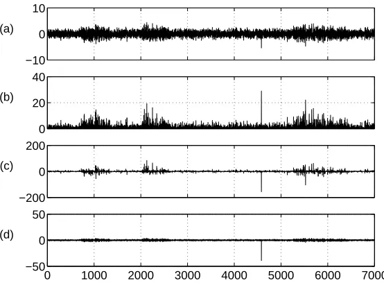
Kurtosis as an objective function is notorious for being prone to overfitting and produc-ing very spiky source estimates (S¨arel¨a and Vig´ario, 2003, Hyv¨arinen, 1998). For illustration of this consider Fig. 3. There one iteration of DSS using kurtosis based denoising is shown. Assume that via some means source estimate shown in Fig. 3a has been reached. The source seems to contain increased activity in three portions (around time instances 1000, 2300 and 6000). It as well contains a peak roughly at time instance 4700. The signal vari-ance estimate,i.e., the mask is shown in Fig. 3b. While it has boosted somewhat the broad activity compared to the silent parts, the magnification of the peak is far greater. Thus the denoised source estimate s+ (Fig 3c) has nearly nothing else than the peak. The new source estimatesnew, based on the new projection wnew, is a clear spike having little left of the broad activity.
−10 0 10 (a)
0 20 40 (b)
−200 0 200 (c)
0 1000 2000 3000 4000 5000 6000 7000 −50
0 50 (d)
The denoising interpretation suggests that the failure to extract the broad activity is due to a poor estimate of SNR.
3.2.2 Better estimate for the signal variance
Let us now consider a related but better founded estimate. Assuming that s is composed of Gaussian noise with a constant variance σn2 and Gaussian signal with non-stationary varianceσ2
s(t), the maximum-a-posteriori (MAP) estimate of the signal is
s+(t) =s(t) σ 2
s(t)
σ2tot(t), (26)
whereσ2
tot(t) =σs2(t) +σn2(t) is the total variance of the observation.
The kurtosis based DSS (25) can be acquired from this MAP estimate if the signal variance is assumed to be far smaller than the total variance. In that case it is reasonable to assume σ2
tot to be constant and σs2(t) can be estimated by s2(t)−σn2. Subtraction of
σn2 does not affect the fixed points as it can be embedded in the termβ(s) = −σn2/σtot in Eq. (21) as will be argued in Sec. 4.3. Likewise, division byσ2tot(t) is absorbed byα(s).
Comparison of Eq. (26) and Eq. (25) immediately suggests improvements to the kurtosis based DSS. For instance, it is clear that ifs2(t) is large enough, it is not reasonable to assume that σ2s(t) is small compared to σn2(t). Instead, the mask should saturate for large s2(t). This already improves robustness against outliers and alleviates the tendency to produce spiky source estimates.
We suggest the following improvements over kurtosis based denoising function (25):
1. The estimates of signal variance and total variance are based on several observations. The rationale of smoothing is the assumption of smoothness of the signal variance. In practice this can be achieved by low-pass filtering the time, frequency or time-frequency description ofs2(t) yielding the approximation of total variance.
2. The noise variance is likewise estimated from data. It should be some kind of soft minimum of the estimated total variances because the estimate can be expected to have random fluctuations. We suggest the following formula:
σ2n=C¡
exp{E[logσn2+σ2tot(t)]} −σ2n¢
. (27)
The noise variance σ2n appears on both sides of the equation, but at the right-hand side, it appears only to prevent rare small values of σ2tot from spoiling the estimate. Hence, we used the previously estimated value on the right-hand side. The constant C is tuned such that the formula gives a consistent estimate of the noise variance if the source estimate is, in fact, nothing but Gaussian noise.
3. The signal variance should be close to the estimate of the total variance minus the estimate of the noise variance. Since a variance cannot be negative and the estimate of the total variance has fluctuations, we use a formula which yields zero only when the total variance is zero but which asymptotically approaches σtot2 (t)−σ2n for large values of the total variance:
σs2(t) =
q
σ4
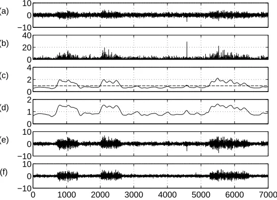
As an illustration of these improvements consider Fig. 4 where one iteration of DSS using the MAP estimate is shown. The first two subplots (Fig. 4a and b) are identical to the ones using kurtosis based denoising. In Fig. 4c, the energy estimate is smoothed using low-pass filtering. Note that the broad activity has been magnified when compared to the spike around time instance 4700. The noise level σ2n, calculated using Eq. (27), is shown in dashed line. Corresponding masking (Fig. 4d) results in a denoised source estimate using Eq. (26), shown in Fig. 4e. Finally, the new source estimatesnew is shown after five iterations of DSS in Fig. 4f. DSS using the MAP-based denoising has clearly removed a considerable amount of background noise as well as the lonely spike.
−10 0 10 (a)
0 20 40 (b)
0 2 4 (c)
0 1 2 (d)
−10 0 10 (e)
0 1000 2000 3000 4000 5000 6000 7000 −10
0 10 (f)
Figure 4: a) Source estimatesb)s2(t)c) Smoothed total energy with the noise level in dashed line d) Denoising mask e) Denoised source estimate s+ f ) Source estimate after five iterations of DSS.
The exact details of these improvements are not crucial, but we wanted to show that the denoising interpretation of Eq. (25) can carry us quite far. The above estimates plugged into Eq. (26) yield a DSS algorithm which is far more robust against overfitting, does not produce the spiky signal estimates and in general yields signals with better SNRs than kurtosis.
Despite the merits of the DSS algorithm described above, there is still one problem with it. While the extracted signals have excellent SNR, they do not necessarily correspond to independent sources,i.e., the sources may remain mixed. This is because there is nothing in the denoising which could discard other sources. Assume, for instance, that two sources have clear-cut and non-overlapping times of strong activity (σ2
s(t)À 0) and remain silent
Denoising can thus clean the noise from the signal estimate, but it cannot decide between the two sources.
In this respect, kurtosis actually works better than DSS based on the above improve-ments. This is because the mask never saturates and small differences in the strengths of the relative contributions of two original sources in the current source estimate will be amplified. The problem only occurs in the saturated regime of the mask and we therefore suggest a simple modification of the MAP estimate (26):
ft(s) =s(t)
σ2sµ(t)
σ2 tot(t)
, (29)
whereµis a constant slightly greater or equal to one. Note that this modification is usually needed at the beginning of the iterations only. Once the source estimate is dominated by one of the original sources and the contributions of the other sources fall closer to the noise level, the values of the mask are smaller for the other original sources possibly still present in the estimated source.
Another approach is based on the finding that the orthogonalisation of the projection vectors W cancels only the linear correlation between different sources. Higher-order cor-relations may still exist. For instance, the variances of different sources can be correlated. Schwartz and Simoncelli (2001) have suggested that variances may be decorrelated by a divisive procedure, in contrast to the orthogonalisation of W, a subtractive procedure. Then it is necessary to estimate explicitly the correlation between one source and the other sources in the current source estimate. The estimate of the total variance can be based in σtot2 (t) =σ2s(t) +σn2(t) +σothers2 (t), where σothers2 (t) stands for the estimate of total leakage of variance from the other sources. This approach has been further pursued by Valpola and S¨arel¨a (2004).
The problems related to kurtosis are well known and several other improved nonlinear functionsf(s) have been proposed. However, some aspects of the above denoising, especially smoothing of the total-variance estimates2(t), have not been suggested previously although they arise quite naturally from the denoising interpretation.
3.2.3 Tanh-nonlinearity interpreted as saturated energy estimate
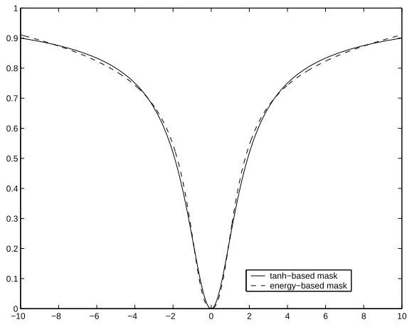
A popular replacement of the kurtosis-based nonlinearity (25) is the hyperbolic tangent tanh(s) operating point-wise for the sources. It is generally considered to be more robust against overfitted and spiky source estimates than kurtosis. By selecting α(s) = −1 and β(s) = 1, we arrive at
ft(s) =s(t)−tanh[s(t)] =s(t) µ
1−tanh[s(t)] s(t)
. (30)
Now the term multiplying s(t) can be interpreted as a mask related to SNR. Unlike the na¨ıve mask s2(t) resulting from kurtosis, the tanh-based mask (30) saturates, though not very fast.
−100 −8 −6 −4 −2 0 2 4 6 8 10 0.1
0.2 0.3 0.4 0.5 0.6 0.7 0.8 0.9 1
tanh−based mask energy−based mask
Figure 5: The tanh-based denoising mask 1−tanh(s)/s is shown together with the energy-based denoising mask proposed here. The parameters in the proposed mask were
σ2n = 1 and µ = 1.08. We have scaled the proposed mask to match the scale of the tanh-based mask.
we propose are thatσ2
ncan be tuned to the source estimate,µcan be controlled during the
iterations and the estimate of the signal energy can be smoothed. These features contribute to the resistance against overfitting and spiky source estimates.
3.3 Other denoising functions
There are cases where the system specification itself suggests some denoising schemes. One such case is described in Sec. 5.6. Another example is source separation with a micro-phone array combined with speech recognition. Many speech recognition systems rely on generative models which can be readily used to denoise the speech signals.
Sometimes the sources can be grouped to form interesting subspaces. This could hap-pen, e.g., when all the sources are not independent of each others, but there exists anyway subspaces that are mutually independent. Some form of subspace rules can be used to guide the extraction of interesting subspaces in DSS. It is possible to further relax the indepen-dence criterion at the borders of the subspaces. This can be achieved by incorporating a neighbourhood denoising rule in DSS, resulting in a topographic ordering of the sources. One such topographic rule was used in topographic ICA (Hyv¨arinen et al., 2001a).
It is possible to combine various denoising functions when the sources are characterised by more than one type of structure. Note that the combination order might be crucial for the outcome. This is simply because, in general,fi(fj(s))6=fj(fi(s)) wherefiandfjpresent
two different linear or nonlinear denoisings. As an example, consider the combination of the linear on/off-mask (22) and (23), and the nonlinear energy based mask (29): the noise estimation becomes significantly more accurate when the on/off-masking is performed only after the nonlinear denoising.
Finally, a source might be almost completely known. Then it is possible to apply a detailed matched filter to estimate the mixing coefficients or the noise level. Detailed matched filters have been used in Sec. 5.1 to get an upper limit of the SNRs of the source estimates.
4. Approximation for the objective function
The virtue of DSS framework is that it allows one to develop procedural source separation algorithms without referring to an exact objective function. However, in many cases an ap-proximation of the objective function is nevertheless useful. In this section, we propose such an approximation and discuss its uses, including monitoring and acceleration of convergence as well as analysis of separation results.
4.1 Derivation of the approximation
As shown in Sec. 2.1, Eq. (13), the objective function corresponding to linear denoising f(s) =sD∗ isgs(s) =sD∗sT, given thatD∗ is a symmetric matrix6. This can be written as gs(s) =s flinT (s).This formula is exact for linear DSS and we propose it as an approximation ˆ
gs for the objective function for nonlinear DSS as well:
ˆ
gs(s) =s fT(s). (31)
There is, however, an important caveat to be made. Note that Eq. (21) includes the scalar functions α(s) and β(s). This means that functionally equivalent DSS algorithms can be implemented with slightly different denoising functionsf(s) and while they would converge exactly to the same results, the approximation (31) might yield completely different values. In fact, by tuning α(s), β(s) or both, the approximation ˆgs(s) could be made to yield any desired function h(s) which needs have no correspondance to the truegs(s).
Due toα(s) andβ(s), it seems virtually impossible to write down a simple approximation ofgs(s) that could not go wrong with a malevolent choice off(s). In the following, however, we argue that Eq. (31) is in most cases a good approximation and it is usually easy to check
whether it behaves as desired—yields values which are monotonic in SNR. If it doesn’t, α(s) andβ(s) can be easily tuned to correct this.
Let us first check what would be the DSS algorithm minimising ˆgs(s). Obviously, the approximation is good if the algorithm turns out to use a denoising similar tof(s). Substi-tutings=wTX in Eq. (31) and deriving the DSS algorithm corresponding to ˆgs similarly as in Eqs. (17)–(18) results in:
w+ =X[fT(s) +JT(s)sT], (32) where J is the Jacobian of f. This should conform with the corresponding steps in the nonlinear DSS (16) and (11) which uses f(s) for denoising. For this to be ture, the two terms in the square brackets should have the same form,i.e.,f(s)∝s J(s).
As expected, in the linear case the two algorithms are exactly the same because the Jacobian is a constant matrix andf(s) =sJ. The denoised sources are also proportional to s J(s) in some special nonlinear cases, for instance, whenf(s) =sn.
As an example of how Eq. (31) can fail to approximate the true objective function, consider the masking based denoisings discussed in Section 3 where denoising is implemented by multiplying the source point-wise by a mask. This means that according to Eq. (31), g(s) will be a sum ofs2(t) weighted by the values of the mask. If the mask is constant w.r.t. s, denoising is linear and Eq. (31) is an exact formula, but let us assume that the mask is computed based on the current source estimates.
In some cases it may be useful to normalise the mask and this could be implemented in several ways. Some possiblities that may come to mind are to normalise the maximum value or the sum of squared values of the mask. While this type of normalisation has no effect on the behaviour of DSS, it can render the approximation (31) useless. This is because a maximally flat mask usually corresponds to a source with a low SNR. However, after normalisation, the sum of values in the mask would be greatest for a maximally flat mask and this tends to produce high values of the approximation ofg(s) conflicting the low SNR. As a simple example, consider the mask to be m(t) = s2(t). This corresponds to the kurtosis-based denoising (25). Now the sum of squared values of the mask is P
s4(t), but so is sfT(s). If the mask were normalised by dividing by the sum of squares, the approximation (31) would always yield a constant value of one, totally independent ofs.
A better way of normalising a mask is to normalise the sum of the values. Then Eq. (31) should always yield approximately the same value if the mask and source estimate are unrelated, but the value would be greater for cases where the magnitude of the source is correlated with the value of the mask. This is usually a sign of a structured source and consequently a high SNR.
4.2 Negentropy ordering
The approximation (31) can be readily used for monitoring the convergence of DSS algo-rithms. It is always easy to use it for ordering the sources based on their SNR if several sources are estimated using DSS with the same f(s). However, simple ordering based on Eq. (31) is not possible if different denoising functions are used for different sources.
is a measure of disorder and is dependent on the variance of the variable. Negentropy is a normalised quantity measuring the difference between the differential entropy of the component and a Gaussian component with the same variance. Negentropy is zero for the Gaussian distribution and non-negative for all distributions since among the distributions with a given variance, the Gaussian distribution has the highest entropy.
Calculation of the differential entropy assumes the distribution to be known. Usually this is not the case and the estimation of the distributions is often difficult and computationally demanding. Following Hyv¨arinen (1998), we approximate the negentropy N(s) by
N(s) =H(ν)−H(s)≈ηg[ˆgs(s)−gˆs(ν)]2, (33)
where ν is a normally distributed variable. The reasoning behind Eq. (33) is that ˆgs(s) carries information about the distribution of s. If ˆgs(s) equals ˆgs(ν), there is no evidence of the negentropy to be greater than zero, so this is when N(s) should be minimised. A Taylor series expansion of N(s) w.r.t. ˆgs(s) around ˆgs(ν) yields the approximation (33) as the first non-zero term.
Comparison of signals extracted with different optimisation criteria presumes that the weighting constantsηgshould be known. We propose thatηgcan be calibrated by generating
a signal with a known, nonzero negentropy. Negentropy ordering is most useful for signals which have a relatively poor SNR—the signals with a good SNR will most likely be selected in any case. Therefore we choose our calibration signal to have SNR of 0 dB,i.e., it contains equal amounts of signal and noise in terms of energy: ss = (ν +sopt)/√2, where sopt is a pure signal having no noise. It obeys fully the signal model implicitly defined by the corresponding denoising functionf. Sincesopt andν are uncorrelated,sshas unit variance.
The entropy of ν/√2 is
H(ν/√2) =H(ν) + log 1/√2 =H(ν)−1/2 log 2. (34)
Since the entropy can only increase by adding a second, independent signal sopt,H(ss)≥ H(ν)−1/2 log 2. It thus holdsN(ss) =H(ν)−H(ss)≤1/2 log 2. One can usually expect thatsopt has a lot of structure,i.e., its entropy is low. Then its addition toν/√2 does not significantly increase the entropy. It is therefore often reasonable to approximate
N(ss)≈1/2 log 2 = 1/2 bit, (35)
where we chose base-2 logarithm yielding bits. Depending on sopt, it may also be pos-sible to compute the negentropy of N(ss) exactly. This can then be used instead of the
approximation (35).
The coefficients ηg in Eq. (33) can now be solved by requiring that the
approxima-tion (33) yields Eq. (35) forss. This results in
ηg =
1
2(ˆg(ss)−ˆg(ν))2
bit (36)
and finally, substitution of the approximation of the objective function (31) and Eq. (36) into Eq. (33) yields the calibrated approximation of the negentropy:
N(s)≈
£
s fT(s)−νfT(ν)¤2
2 [ssfT(ss)−νfT(ν)]2
4.3 Spectral shift
In the classical power method, the convergence speed depends on the ratio of the largest eigenvalues,|λ1/λ2|, where|λ1|>|λ2|. If this ratio is close to unity, the matrix multiplica-tion (4) does not promote the largest eigenvalue effectively compared to the second largest eigenvalue.
The convergence speed in such cases can be increased by so called spectral shift7 which modifies the eigenvalues without changing the fixed points. At the fixed point of the linear DSS,
λw=XflinT (s). (38) Then it also holds that (λ+λβ)w=Xflin(s)T+λβwfor anyλβ. The additional term simply
addsλβ to all eigenvalues. The spectral shift modifies the ratio of two largest eigenvalues8
which becomes|(λ1+λβ)/(λ2+λβ)|>|λ1/λ2|, provided thatλβ is negative but not much
smaller than −λ2. This can greatly increase the convergence speed of the classical power method.
However, for very negative λβ, some eigenvalues will become negative. In fact, if λβ is
small enough, the absolute value of the originally smallest eigenvalue will exceed that of the originally largest eigenvalue. Iterations of linear DSS will then minimise the eigenvalue rather than maximise it. It does not seem very useful to minimiseg(s), a function that mea-sures the SNR of the sources. But as we saw with negentropy and the approximation (33) of it, values g(s) < g(ν) are, in fact, indicative of signal. A reasonable selection for λβ is
thus−νflinT (ν) which leads linear DSS to extremiseg(s)−g(ν) or, equivalently, to maximise the negentropy approximation (33).
A side effect for this type of spectral shift is that the estimatewof the principal direction changes its sign at each iteration if the eigenvalue is negative. This needs to be kept in mind when determining the convergence of DSS.
Above, the spectral shift has been applied to the eigenvalues of the matrix ZZT. How-ever, in DSS the spectral shift can be embedded in the denoising of the source using β(s) according to Eq. (21) because β(s) =λβ/T. From now on, we use β(s) to implement the
spectral shift.
Unlike in linear DSS, the approximation (31) may not accurately represent the objective function in nonlinear DSS. Consequently, nonlinear DSS does not necessarily optimise the eigenvalues λdefined by Eq.(38). As we argued before, Eq. (31) nevertheless offers a good approximation ˆgs(s). Hence we suggest a spectral shift
β =−gˆs(ν)/T (39)
for nonlinear DSS, too. One way to improve the efficiency of this approach is to try to scale the denoising such that a Gaussian noise signal always has a similar contribution in the denoised signal. For example, if the denoising is implemented by masking the source signal, the contribution of a fixed amount of Gaussian noise to the denoised source signal can be equalised by normalising the sum of the masking components.
7. The set of the eigenvalues is often called eigenvalue spectrum.
It is not necessary to base the spectral shift on a global approximation of gs(ν). An alternative is to linearisef(s) around the current source estimatesand use this to compute β(s) as follows:
ˆ
f(ν) =f(s) + (ν−s)J(s) (40)
β(s) =−ˆgs(ν)/T =−ν[f(s) + (ν−s)J(s)]T/T
=−trJ(s)/T (41)
The last step follows from the fact that the elements ofν are mutually uncorrelated and have zero mean and unit variance. If denoising is instantaneous, f(s) = [f1(s(1))f2(s(2)) . . .], the shift can be written as β = −P
tft0(s(t))/T. This is the spectral shift used in
Fas-tICA (Hyv¨arinen, 1999), but it has been justified as an approximation to Newton’s method and our analysis thus provides a novel interpretation.
In general, iterations converge faster with the FastICA-type spectral shift (41) than with the fixed shift (39) but the latter has the benefit that no gradients need to be computed. This is important when the denoising is defined by a complex nonlinear procedure such as median filtering.
A well known example where the spectral shift by the eigenvalue of a Gaussian signal is useful is the mixture of both super- and sub-Gaussian distributions. DSS algorithm designed for super-Gaussian distributions would lead to λ > λG for super-Gaussian and λ < λG for
sub-Gaussian distributions, λG being the eigenvalue of the Gaussian signal. By shifting the
eigenvalue spectrum by−λG, the most non-Gaussian distributions will result in the largest
absolute eigenvalues regardless of whether the distribution is super- or sub-Gaussian. By using the spectral shift it is therefore possible to extract both super- and sub-Gaussian distributions with a denoising scheme which is designed for one type of distributions only.
Consider for instance f(s) = tanhs which can be used as denoising for sub-Gaussian signal while, as we saw before, s−tanhs=−(tanhs−s) is a suitable denoising for super-Gaussian signals. This shows that depending on the choice of β, DSS can find either sub-Gaussian (β = 0) or super-Gaussian (β = −1) sources. With the FastICA spectral shift (41), β will always lie in the range −1< β ≤tanh21−1≈ −0.42. In general, β will be closer to −1 for super-Gaussian sources which shows that FastICA is able to adapt its spectral shift to the source distribution.
None of the above methods always work for nonlinear DSS. Sometimes the spectral shift turns out to be either too modest or strong, leading to slow convergence or lack of convergence, respectively. For this reason, we suggest a simple stabilisation rule: instead of updatingw intownew defined by (12), it is updated into
wadapted= orth(w+γ∆w) (42)
∆w=wnew−w, (43)
techniques considered above, and some additional ones, are studied further in Valpola and S¨arel¨a (2004).
Sometimes there are several signals with similar large eigenvalues. It may then be impossible to use spectral shift to accelerate their separation significantly because of small eigenvalues that would assume very negative values exceeding the signal eigenvalues in magnitude. In that case, it may be beneficial to first separate the subspace of the signals with large eigenvalues from the smaller ones. Spectral shift will then be useful in the signal subspace.
4.4 Detection of overfitting
In exploratory data analysis DSS is very useful for giving a better insight to the data using a linear factor model. However, it is possible that DSS extracts structures that are not actually present in the data but are generated by the denoising function, i.e., the results may be due to overfitting.
Overfitting in ICA has been extensively studied by S¨arel¨a and Vig´ario (2003). It was observed that it typically results in signals that are mostly inactive, except for a single spike. In DSS the outlook of the overfitted results depends on the denoising criterion. The results of exploratory DSS should thus be treated with a healthy amount of scepticism.
To detect an overfitted result, one should know how it looks like. As a first approxima-tion, DSS can be performed with same amount of i.i.d Gaussian data. Then all the results present cases of overfitting. Even better characterisation of the overfitting results can be obtained by mimicking the actual data characteristics as well as possible. In that case it is important to make sure that the structure assumed by the signal model has been broken. Both the Gaussian overfitting test and the more advanced test are used throughout the experiments in Secs. 5.2–5.5.
Note that in addition to visual test, the methods described above provide us with a quantitative measure as well. Using the negentropy approximation (37), we can set a threshold under which the sources are very likely overfits and do not carry much real struc-ture. In the simple case of linear DSS, the negentropy can be approximated easily using the corresponding eigenvalue.
5. Experiments
5.1 Artificial signals
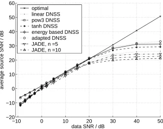
Artificial signals were mixed to compare different DSS schemes and JADE (Cardoso, 1999). Ten mixtures of the five sources were produced and independent white noise was added with different SNRs ranging from nearly noiseless mixtures of 50dB to -10dB, a very noisy case. The original sources and the mixtures are shown in Figs. 6a and 6b respectively. The mixtures shown have SNR of 50 dB.
(a) (b)
Figure 6: (a) Five artificial signals with simple frequency content (signals #1 and #2), simple on/off non-stationarity in time domain (signals #3 and #4) or quasi-periodicity (signal #5). (b) Ten mixtures of the signals in (a).
5.1.1 Linear denoising
In this section, we show how the simple linear denoising schemes described in Sec. 3.1 can be used to separate the artificial sources. These schemes require prior knowledge about the source characteristics.
The base frequencies of the first two signals were assumed to be known. Thus two band-pass filtering masks were constructed around these base frequencies. The third and fourth source estimates were known to have periods of activity and non-activity. Third was known to be active in the second quadrant and the fourth a definite period in the latter half. They were denoised using binary masks in time domain. Finally, the fifth source had a known quasi-periodic repetition rate and was denoised using the averaging procedure described in Sec. 3.1.4 and Fig. 2. Since all the five denoisings are linear, five separate filtered data sets were produced and PCA was used to recover the principal components. The separation results are described in Sec. 5.1.3 together with the results of other DSS schemes and JADE.
5.1.2 Nonlinear exploratory denoising
the original signals. The author did not receive any additional information, so he was forced to apply a blind approach. He chose to use the masking procedure based on the instantaneous energy estimate, described in Sec. 3.2. To enable the separation of both sub-and super-Gaussian sources in the MAP-based signal-variance-estimate denoising, he used the spectral shift (39). To ensure convergence, he used the 179-rule to control the step size γ (42). Finally, he did not smooth s2(t) but used it directly as the estimate of the total instantaneous varianceσ2tot(t).
Based on the separation results of the variance-based DSS, he further devised specific masks for each of the source. He chose to denoise the first source in frequency domain with a strict band-pass filter around the main frequency. The author decided to denoise the second source by a simple denoising function f(s) = sign(s). This makes quite an accurate signal model though it neglects the behaviour of the source in time. The third and fourth signal seemed to have periods of activity and non-activity. He found an estimate for the active periods by inspecting the instantaneous variance estimates s2, and devised simple binary masks. The last signal seemed to consist of alternating positive and negative peaks with fixed inter-peak-interval as well as some additive Gaussian noise. The signal model was tuned to model the peaks only.
5.1.3 Separation results
In this section, we compare the separation results of the linear denoising (Sec. 5.1.1), variance-based denoising and adapted denoising (Sec 5.1.2) to other DSS algorithms. In particular, we compare to the popular denoising schemes f(s) = s3 and f(s) = tanh(s), suggested for use with FastICA (1998). We compare to JADE (Cardoso, 1999) as well. During sphering in JADE, the number of dimensions were either reduced (n= 5) or all the ten dimensions were kept (n= 10).
We restrained from using deflation in all the different DSS schemes to avoid suffering from cumulative errors in separation of the first sources. Instead one source was extracted with each of the masks several times using different initial vector w until five sufficiently different source estimates were reached (see Himberg and Hyv¨arinen, 2003, Meinecke et al., 2002, for further possibilities along these lines). Deflation was only used if no estimate could be found for all the 5 sources. This was often the case for poor SNR under 0dB.
To get some idea of statistical significance of the results, each algorithm was used to separate the sources ten times with the same mixtures, but different measurement noises. The average SNRs of the sources are depicted in Fig. 7. The straight line above all the DSS schemes represents the optimal separation. It is achieved by calculating the unmixing matrix explicitly using the true sources.
−10 0 10 20 30 40 50 −20
−10 0 10 20 30 40 50 60
data SNR / dB
average source SNR / dB
optimal linear DNSS pow3 DNSS tanh DNSS
energy based DNSS adapted DNSS JADE, n =5 JADE, n =10
Figure 7: Average SNRs for the estimated sources averaged over 10 runs.
optimal one and the lower group consists of the blind approaches. This seems reasonable, since it makes sense to rely more on prior knowledge when the data is very noisy.
5.2 Exploratory source separation in rhythmic MEG data
In biomedical research it is usual to design detailed experimental frameworks to examine in-teresting phenomena. Hence it offers a nice field of application for both blind and specialised DSS schemes. In the following we test the developed algorithms in signal analysis of magne-toencephalograms (MEG, H¨am¨al¨ainen et al., 1993). MEG is a completely non-invasive brain imaging technique measuring the magnetic fields on scalp caused by syncronous activity in the cortex.
her eyes open. The data has been sampled with fs = 200 Hz, and there are T = 65536
time samples giving total of more than 300 seconds of measurement. The magnetic fields are measured using a 122-channel MEG device. Some source separation results of this data have been reported by S¨arel¨a et al. (2001). Prior to any analysis, the data is high-pass filtered with cut-off frequency of 1 Hz, to get rid of the dominating very low frequencies.
5.2.1 Denoising in rhythmic MEG
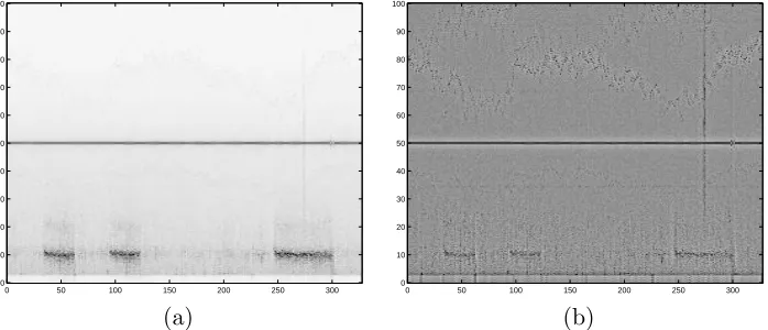
Examination of the average spectrogram in Fig. 8a reveals clear structures indicating the existence of several, presumably distinct, phenomena. The burst-like activity around 10 Hz and the steady activity at 50 Hz dominate the data, but there seem to be some weaker phenomena as well, e.g., on higher frequencies than 50 Hz. To amplify these, we not only sphere the data spatially but temporally as well. This temporal decorrelation actually makes the separation harder, but enables the finding of the weaker phenomena. The normalised and filtered spectrogram is shown in Fig. 8b.
0 50 100 150 200 250 300
0 10 20 30 40 50 60 70 80 90 100
0 50 100 150 200 250 300
0 10 20 30 40 50 60 70 80 90 100
(a) (b)
Figure 8: (a) Averaged spectrogram of all the 122 MEG channels. (b) Frequency normalised spectrogram.
The spectrogram data seems well suited for demonstrating the exploratory data analysis use of DSS. As some of the sources seem to have quite steady frequency content in time, but others changing in time, we used two different time-frequency-analyses as described in Sec. 3.1.3 with lengths of the spectraTf = 1 and Tf = 256. The first spectrogram is then
actually the original frequency-normalised and filtered data with only time information. We apply the several noise reduction principles based on the estimated variance of the signal and the noise discussed in Sec. 3.2. Specifically, the power spectrogram of the source estimate is smoothed over time and frequency using 2-D convolution with Gaussian windows. The standard deviations of the Gaussian windows wereσt= 8/π and σf = 8/π.
until µ <1 is reached. Finally, the new projection vector is calculated using the stabilised version (42), (43) with the 179-rule in order to ensure convergence.
5.2.2 Separation results
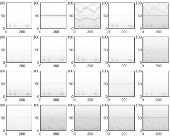
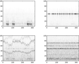
The separated signals, depicted in Fig. 9, include several interesting sources. Due to poor contrast in Fig. 9, we show enhanced and smoothed spectrograms of selected interesting, but low contrast, components (#1, #2, #3 and #18) in Fig. 10. In the rest of this paper, we always show the enhanced spectrograms of extracted components. First of all, there exist several sources with α-activity (#1, #4 and #7 for example). The second and 6th source are clearly related to the power-line. The fourth source depicts an interesting signal caused probably by some anomaly in either the measuring device itself or its physical surroundings. In source #18, there is another, presumably artefactual source, composed of at least two steady frequencies around 70 Hz.
0 200 0 50 100 0 200 0 50 100 0 200 0 50 100 0 200 0 50 100 0 200 0 50 100 0 200 0 50 100 0 200 0 50 100 0 200 0 50 100 0 200 0 50 100 0 200 0 50 100 0 200 0 50 100 0 200 0 50 100 0 200 0 50 100 0 200 0 50 100 0 200 0 50 100 0 200 0 50 100 0 200 0 50 100 0 200 0 50 100 0 200 0 50 100 0 200 0 50 100
Figure 9: Spectrograms of the extracted components (comps. 1–5 on the topmost row)
The DSS approach described above seems to be reliable and fast: the temporal decor-relation of the data enabled the finding of very weak sources and yet we found several clear α-sources as well. Valpola and S¨arel¨a (2004) have further studied the convergence speed, reliability and stability of DSS with various speedup methods, such as the spectral shift used in FastICA. Convergence speed exceeding standard FastICA by 50 % was reported.
0 100 200 300 0
20 40 60 80 100
0 100 200 300
0 20 40 60 80 100
0 100 200 300
0 20 40 60 80 100
0 100 200 300
0 20 40 60 80 100
Figure 10: Enhanced and smoothed spectrograms of the selected components (correspond to sources #1, #2, #3 and #18 in Fig. 9)
uncovered by variance-based masking. First we take a look at the α-subspace. Then, in Sec. 5.4 the anomalous signals (bottom row of the Fig. 10) are inspected further. Finally, in Sec. 5.5 we show that with specific knowledge it is possible to find even very weak phenomena in MEG data using DSS.
5.3 Adaptive extraction of the α-subspace
Exploratory source separation revealed several sources with significant activity on the α -band (e.g., #3 and #6). But in previous section, only general noise reduction principles were used. In this section, we further tune the masks to achieve maximal signal to noise ratio in theα-subspace.
5.3.1 Denoising of the α-sources
These two characteristics (10 Hz and 20 Hz frequency content and on/off activity) are directly exploited to make a band-pass filter in the spectrogram (see Sec. 3.1). Since this denoising is completely linear, we have chosen to use the PCA type of DSS, as described by Eqs. (3), (4) and (5).
5.3.2 Separation results
We calculated all the 122 principal components related to theα-masked data. Spectrograms of the components having the 20 largest eigenvalues are shown in Fig. 11. They are in descending order according to corresponding eigenvalues.
0 200 0 50 100 0 200 0 50 100 0 200 0 50 100 0 200 0 50 100 0 200 0 50 100 0 200 0 50 100 0 200 0 50 100 0 200 0 50 100 0 200 0 50 100 0 200 0 50 100 0 200 0 50 100 0 200 0 50 100 0 200 0 50 100 0 200 0 50 100 0 200 0 50 100 0 200 0 50 100 0 200 0 50 100 0 200 0 50 100 0 200 0 50 100 0 200 0 50 100
Figure 11: Spectrograms of the components of the extractedα-subspace (comps. 1–5 on the topmost row).
Thus it is not reasonable to assume that there exists much more than 15 α-components in the data.
5.3.3 Rotation of the α-subspace
There is a wide literature concerning the localisation of MEG and EEG sources (c.f., H¨am¨al¨ainen et al., 1993, Niedermeyer and Lopes da Silva, 1993). Though we do not intend to go into details here, we note that there is little reason to believe that the linear α-mask used above would actually rotate theα-subspace in physiologically meaningful components. It probably only effectively separates between the noise and the signal subspace.
To actually find a meaningful separation, we need an additional criterion for the rotation. Recently, ICA has been suggested for this task by Vig´ario et al. (2000), Jung et al. (2000), Tang and Pearlmutter (2003). It can find a meaningful rotation only in the case where the sources have non-Gaussian distributions. This might easily not be the case in burst-like activity ofα-sources (see Vig´ario et al., 2000, for an example). Furthermore, the separation is not guaranteed even if the distributions are non-Gaussian. For instance, the rotational ambiguity of a sine and a cosine remains even if they are modulated with envelopes, if the envelopes are similar enough.
Another possible approach, more in lines with the philosophy of this paper, is to find properties that the sources might differ in. One interesting possibility is to consider further rotation of the α-subspace by the mutual strengths of the base frequence (10 Hz) and first harmonics (20 Hz) of theα-activity.
We propose to achieve the rotation by another linear DSS scheme in the resphered α -subspace of 16 α-related components, where only the active portions in time have been preserved. The denoising is based on band-pass filtering around 20 Hz. From the results shown in Fig. 12 it can be seen that the first components have the highest amount of 20 Hz compared to the 10 Hz. Similarly, the last components are ones having the least amount of 20 Hz.
5.4 Adaptive extraction of artefacts
Exploratory DSS separated some presumable artefacts as well. In Fig. 9, the 5th component has a curious wandering frequency around 30–40 Hz and some higher harmonics. Another interesting phenomenon is seen in the 14th component, with its steady frequencies around 60 Hz. In this section we adaptively maximise SNR of these signals. We as well check whether some weaker, related signals come forward when the masks are adapted.
5.4.1 Denoising of the steady frequency components
0 200 0 50 100 0 200 0 50 100 0 200 0 50 100 0 200 0 50 100 0 200 0 50 100 0 200 0 50 100 0 200 0 50 100 0 200 0 50 100 0 200 0 50 100 0 200 0 50 100 0 200 0 50 100 0 200 0 50 100 0 200 0 50 100 0 200 0 50 100 0 200 0 50 100 0 200 0 50 100
Figure 12: Spectrograms of the components of the rotated α-subspace (comps. 1–4 on the topmost row).
5.4.2 Separation results
Using the adaptive procedure described above, 16 components were reached. Some of them are highly mutually correlated because their corresponding masks are similar. The data seemed to have a total of four different components uncorrelated to each others. The spectra and the spectrograms of the different components found are shown in Fig. 13. The first two are quite similar, having steady frequency around 34 Hz. Likewise, the last two signals have similar frequency content having several steady higher frequencies, mainly on band 60–75 Hz.
5.4.3 Denoising of the wandering frequency components
For the wandering signal (bottom left in Fig. 10), we adaptively tune a mask in the time-frequency-space so that it takes into account the slow drifting of the base frequency. The very clear 2nd and 3rd harmonics are used to aid the estimation of the base frequency. Note that the third harmonic surpasses the Nyquist frequency offs/2 = 100 Hz at certain
0 20 40 60 80 100 0
100 200
0 20 40 60 80 100
0 50 100
0 20 40 60 80 100
0 100 200
0 20 40 60 80 100
0 50 100
frequency / Hz
0 100 200 300
0 20 40 60 80 100
0 100 200 300
0 20 40 60 80 100
0 100 200 300
0 20 40 60 80 100
0 100 200 300
0 20 40 60 80 100 (a) (b)
Figure 13: (a) Power spectra of the components having several steady frequencies. (b) Smoothed spectrograms of the corresponding components (comps. 1–2 on the topmost row).
5.4.4 Separation results
Using the DSS procedure described above, we extracted several signals having wandering frequency around 30–40 Hz and higher harmonics. Two of these are shown in Fig. 14. As the tuned mask is a very narrow one, it can see similar structure in pure Gaussian data already. Comparison of the corresponding eigenvalues revealed that all the other extracted wandering components, expect for the two shown, are caused by overfitting. The base frequency of the second source is not clearly visible but this appears to be caused by greater noise variance on the frequencies compared to the higher frequencies where the harmonics are.
0 50 100 150 200 250 300
0 10 20 30 40 50 60 70 80 90 100
0 50 100 150 200 250 300
0 10 20 30 40 50 60 70 80 90 100 (a) (b)