Improving Voltage Stability Margin Using Voltage Profile and
Sensitivity Analysis by Neural Network
M. R. Aghamohammadi*, S. Hashemi** and M. S. Ghazizadeh*
Abstract: This paper presents a new approach for estimating and improving voltage
stability margin from phase and magnitude profiles of bus voltages using sensitivity analysis of Voltage Stability Assessment Neural Network (VSANN). Bus voltage profile contains useful information about system stability margin including the effect of load-generation pattern, line outage and reactive power compensation, so it is adopted as input pattern of VSANN. In fact, VSANN establishes a functionality for VSM with respect to voltage profile. Sensitivity analysis of VSM with respect to voltage profile and reactive power compensation extracted from information stored in the weighting factor of VSANN is the most dominant feature of the proposed approach. Sensitivity of VSM helps one to select the most effective buses for reactive power compensation aimed enhancing VSM. The proposed approach has been applied to IEEE 39-bus test system which demonstrated applicability of the proposed approach.
Keywords: Voltage Stability Margin, Voltage Profile, Feature Extraction, Neural
Networks, Sensitivity Analysis.
1 Introduction1
Voltage stability is a fundamental component of dynamic security assessment and it has been emerged as a major concern for power system security and a main limit for loading and power transfer. Voltage stability is usually expressed in term of stability margin, which is defined as the difference between loadability limit and the current operating load level. Traditionally, static voltage stability is analyzed based on the power flow model [1]. Several major voltage collapse phenomena resulted in widespread blackouts [2]. A number of these collapse phenomena were reported in France, Belgium, Sweden, Germany, Japan, and the United States [3,4]. Voltage collapse is basically a dynamic phenomenon with rather slow dynamics in time domain from a few seconds to some minutes or more [5]. It is characterized by a slow variation at system operating point due to the load increase and gradual voltage decrease until a sharp change occurs.
In spite of dynamical nature of voltage instability, static approaches are used for its analysis based on the
Iranian Journal of Electrical & Electronic Engineering, 2011. Paper first received 11 May 2010 and in revised form 26 Jan. 2011. * The Authors are with the Department of Electrical Engineering, Power And Water University of Technology, Tehran-Iran.
E-mails: [email protected], [email protected]
** The Author is with the Department of Electrical Engineering, Power And Water University of Technology, Tehran-Iran.
E-mail:[email protected].
fact that the system dynamics influencing voltage stability are usually slow [6-8], so, if system models are chosen properly, the dynamical behavior of power system may be closely approximated by a series of snapshots matching the system conditions at various time steps along the system trajectory [6, 9]. Numerous researches have been devoted to the analysis of both static and dynamic aspects of voltage stability [10]. In order to preserve voltage stability margin at a desired level, online assessment of stability margin is highly demanded which is a challenging task requiring more sophisticated indices. Voltage security assessment could be basically categorized in two types as 1-model based approaches and 2- non model based approaches.
In recent literatures, many voltage stability indices have been presented which are mainly model based approaches evaluated by the load flow calculation. All of the approaches evaluated by sensitivity analysis, continuation power flow [9,11,12], singular value of Jacobian matrix [13,14] and load flow feasibility [6,7] are model based. Some methods utilized system Jacobian matrix [9,12,13,15] by exploiting either its sensitivity or its eigenvalue to determine system vicinity to singularity. All these methods are usually time consuming and not suitable for online applications. In [15] an enhanced method for estimating look-ahead load margin to voltage collapse, due to either saddle-node bifurcation or the limit-induced bifurcation, is proposed.
In [1], a static approach based on optimal power flow (OPF), conventional load flow and singular value decomposition of the load flow Jacobian matrix is proposed for assessing the steady-state loading margin to voltage collapse of the North-West Control Area (NWCA) of the Mexican Power System. In [16], derivative of apparent power against the admittance of load (dS/dY) is proposed for measuring proximity to voltage collapse. The techniques proposed in [2] are able to evaluate voltage stability status efficiently in both pre-contingency and post-contingency states with considering the effect of active and reactive power limits. In [5], based on the fact that the line losses in the vicinity of voltage collapse increase faster than apparent power delivery, so, by using local voltage magnitudes and angles, the change in apparent power flow of line in a time interval is exploited for computation of the voltage collapse criterion. In [17] by means of the singular value decomposition (SVD) of Jacobian matrix the MIMO transfer function of multi-machine power system for the analysis of the static voltage stability is developed. In [18], operating variable information concerning the system base condition as well as the contingency, like line flow, voltage magnitude and reactive reserve in the critical area are used to provide a complex index of the contingency severity. In [8], modal analysis and minimum singular value are used to analyze voltage stability and estimate the proximity of system condition to voltage collapse.
Artificial intelligence techniques have been used in several power system applications. In [15], a feed forward neural network is used to evaluate L index for all buses. In [19] for online voltage stability assessment of each vulnerable load bus an individual feed forward type of ANN is trained. In this method, ANN is trained for each vulnerable load bus and for a wide range of loading patterns. In [20], a neural network-based approach for contingency ranking of voltage collapse is proposed. For this purpose by using the singular value decomposition method, a Radial Basis Function (RBF) neural network is trained to map the operating conditions of power systems to a voltage stability indicator and contingency severity indices corresponding to transmission lines.
In this paper, a novel approach based on neural network application is proposed for online assessment and fast improvement of voltage stability margin. In this method, a voltage stability assessment neural network (VSANN) works as an online voltage stability margin (VSM) estimator and is utilized for enhancing power system’s VSM. In the proposed approach, VSANN is fed by network voltage profile. Network voltage profile obtained by synchronous measurement of bus voltages by means of PMU’s provides an operating feature of power system containing the effects of load-generation pattern, network structure (e.g. line
outage) and reactive power compensation. Therefore, the voltage profile is able to reflect the variation effect of load-generation pattern and network structure (due to line outage) on the voltage stability margin. The easiness of accessibility and measuring of bus voltages demonstrates this approach very suitable for estimating VSM in normal condition and even after being subject to a disturbance.
2 Proposed approach
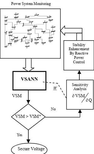
In this paper, for fast estimating and improving voltage stability margin a new approach bade on the application of neural network is proposed. Fig. 1 shows the conceptual structure of the proposed approach. In the proposed approach, at any given operating condition, network voltage profile including both phase and magnitude of bus voltages is provided by synchronous measurement of bus voltages. By feeding the network voltage profile to VSANN, the system VSM corresponding to the current operating point is evaluated. If it is recognized that the system VSM is less than a desired value (VSM*), it will be deduced to enhance the system voltage security. For this purpose by evaluating the sensitivity of VSM with respect to reactive power compensation, the most appropriate buses are found for reactive power compensation. This sensitivity is evaluated by using the information stored in the weighting factors of VSANN during training process and network voltage profile at the current operating condition.
3 Voltage Stability Assessment Neural Network
In this paper, a multilayer feed forward neural network is utilized to map the highly non-linear relationship between network voltage profile and the corresponding voltage stability margin. Network voltage profile provided by synchronous measurement of bus voltages constitutes the input pattern of VSANN. The number of input neurons of VSANN is determined based on the size of the power system to be studied. There is only one output neuron which gives the estimated VSM. The number of hidden neurons is determined based on the trial and error.
Generally, one of the drawbacks of neural network application in power system problems is dependency of its training on the network topology. So, this dependency necessitates updating the training process in the case of any change in network topology due to line outage or line addition. The input pattern of the proposed VSANN is selected in such a way to eliminate the dependency of its training to network topology change which may arise from line or generator outage. Therefore, in the case of line outage, network voltage profile including the effect of network topology, load-generation pattern and reactive power compensation remains as representative of system voltage security.
Fig. 1 Conceptual structure of the proposed approach.
3.1 Training Data
Each training data set corresponds to an operating point of power system and consists of network voltage profile as the input pattern and the associated VSM as the output pattern. In order to train VSANN, it is necessary to prepare sufficient and suitable training data. For this purpose, a wide variety of load-generation increase patterns are adopted. For each load increase pattern denoted as loading pattern, continuation power flow (CPF) calculation is carried out by increasing load and generation through specified steps (i.e. %2) until the point of voltage collapse and loadability limit. Each loading pattern is represented by a vector α with a dimension equal to the number of load buses which shows the trend of load increase on load buses. The element αk, shown by Eq. (1) represents the share of bus
#k for load pick up with respect to the total system load.
loadk
k n
loadk k 1
P
P
α
=
=
∑
(1)Fig. 2 denoted as P-V curve, typically shows bus voltage variation at different operating points toward voltage collapse during increase of load-generation based on a specific loading pattern α.
As shown in Fig. 2, each loading pattern α corresponds to a specific P-V curve and an associated loading limit (Pmax) denoted as loadability limit. During load increase based on a specific loading pattern toward voltage collapse, at different steps of load
increment, system takes various operating points with different corresponding voltage profiles and VSM.
Figure 3 illustrates network voltage profiles evaluated for IEEE 39-bus test system corresponding to different operating points created in the trajectory of a specific load increase pattern until the point of voltage collapse. A voltage profile consists of bus voltages which are arranged according to the bus number. For each operating point with load level Po and with a specific voltage profile, there is a corresponding VSM evaluated by Eq. (2).
o,i max,i o,i
VSM =P - P (2)
where, Pmax,i is system loadability limit associated to the
loading pattern αi and Po,i is system load level at the
operating point.
Loading pattern, generation pattern, network topology and reactive power compensation are the major factors affecting loadability limit and voltage stability margin. In order to embed the effect of network
Fig. 2 Typical P-V curve showing loadability limit and VSM.
Fig. 3 Bus voltage profiles during load increment toward
voltage collapse.
0 0 0.2 0.4 0.6 0.8 1
P (MW)
V
(
p.u
.)
Nose curve
P0 PmaxL.F P
max V.S
0.95 1.05
acceptable operation limits
ALM
VSM
collapse point (Loadability limit)
0 5 10 15 20 25 30 35 40
0 0.2 0.4 0.6 0.8 1
Voltage at collapse point = 0.73926 p.u. loadability limit = 12193.2 MW
V
ol
tag
e (
p.
u.
)
Bus number
No W VSM
Power System Monitoring
Yes
Secure Voltage
VSANN
Stability Enhancement
By Reactive Power Control
VSM > VSM*
Sensitivity Analysis
Q ∂ VSM ∂
topology and reactive power compensation into the voltage profile and training ability of VSANN, for some loading patterns, some lines are taken out and reactive power resources are changed to produce new operating points with associated voltage profiles and VSM for adding to training data. Since voltage profiles are prepared for a wide variation in both extremes of operating conditions including light load and heavy load near to voltage collapse so, VSANN will be able to cover and interpolate all possible variation which may occur in system condition. Therefore, the ability of network voltage profiles for containing the effect of network topology, loading pattern, generation pattern, reactive power compensation and voltage stability margin VSM and also its robustness with respect to changes in system conditions and network topology, are the main motivation for using it as the input pattern for training VSANN. In fact, every unexpected change in system condition creates a corresponding voltage profile which always lays within the extremes voltage profiles and its corresponding VSM can be interpolated by VSANN without failure.
3.2 Feature Extraction
Certain preprocessing steps are performed on the neural network input data and targets to make the training more efficient. The process of eliminating inefficient and redundant data and choosing only those data containing maximum information with respect to the all components of input data is called feature reduction. For training VSANN, the dimension of the input pattern in general is related to the size of power system. The memory requirement and processing time can be reduced either by reducing the dimension of the input data or by reducing the number of training patterns. In this paper, the dimension of input space is reduced by extracting its dominant features in a lower dimension space by using principle component analysis (PCA) [21, 22]. Principle component analysis is one of the well-known feature extraction techniques and a standard technique commonly used for data reduction in statistical pattern recognition and signal processing. PCA is useful in situations where the dimension of the input vector is large, but the components of the vectors are highly correlated.
For this purpose, first the inputs and target are normalized such that they have zero mean and unity standard deviation. This also ensures that the inputs and target fall within a particular range. During the testing phase of VSANN, new inputs are also preprocessed with the mean and standard deviations which were computed for the training set. Then, by applying principal component analysis the normalized input training data are preprocessed. This analysis reduces the size of input pattern by eliminating correlated data and transforms the input data into an uncorrelated space. In
the reduced space, only principle components with more contribution remain. Principal components analysis is carried out using singular value decomposition. PCA can be represented by Equations (3) and (4).
*
11 1i 1n 1
1
*
j1 ji jn i
j
*
k1 ki kn m
k
T T T x
x
T T T * x
x
T T T x
x =
L L
M O M M M
M
L
M O M M
M
L L
(3)
*
k t k m m t
X× =T× * X × (4)
where X is input data consists of phase and magnitude of all bus voltages before feature extraction, T is decomposition and transfer matrix with rows consisting of the eigenvectors of the input covariance matrix and X* is reduced input data including k uncorrelated
components which are ordered according to the magnitude of their variance.
By this transformation, those components contributing by only a small amount to the total variance in the data set are eliminated. Fig. 4 shows the concept and process of feature reduction technique applied to the proposed approach.
3.3 Training VSANN
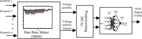
The proposed VSANN is trained by the back-propagation algorithm using Levenberg Marquardt optimization. This algorithm is designed to provide fast convergence. The number of input variables depends on the number of the extracted features of voltage profile. There is only one output neuron representing the estimated VSM. The number of neurons in hidden layer is adopted by trial and error. Early stopping regime is also applied to improve ANN generalization by preventing the training from over fitting problem [23]. In the context of neural network, over fitting is also known as overtraining where further training will not result in better generalization. In this technique, the available data are divided into three subsets. The first subset is the training set which is used for computing the gradient and updating the weighting factors and biases of VSANN. The second subset is the validation set. The error of validation set is periodically monitored during the training process. The validation error will normally decrease during the initial phase of training. When the overtraining starts to occur, the validation error will typically begin to rise. Therefore, it would be useful and time saving to stop the training after the validation error has increased for some specified numbers of iteration. The process of VSANN training consisting of data generation, preprocessing and training is depicted in Fig. 4.
Fig. 4 Conceptual scheme for process of VSANN training.
4 Sensitivity Analysis of VSANN
After training VSANN and in the working mode of the proposed approach shown in Fig.1, if the estimated VSM by VSANN is found out to be less than a desired VSM, it will become necessary to enhance the system stability margin by reactive power compensation. For this purpose, the sensitivity analysis of VSM with respect to bus voltages is performed to find the most effective buses for compensation. The sensitivity of VSM with respect to each bus voltage magnitude can be calculated by Eq. (5) [22] using information stored in the weighting factors of VSANN and input data.
∑NH ∑
1 = i
n
1 = j 1 o i i i 2 o u
) ) u ,j ( T * ) j ,i ( W ( * ) r ( r
∂ ∂
* ) i ( W ( * ) E ( E
∂ ∂
= V
∂
VSM
∂ ψ ϕ
(5)
where:
NH: Number of hidden neurons. n: Number of network buses.
W1(i,j): Weighting factor connecting the jth input neuron
to the ith hidden neuron.
W2(i): Weighting factor connecting output neuron to the
ith hidden neuron.
ri, φi: Input and output of the ith hidden neuron,
respectively.
E, ψ: Input and output of the output neuron, respectively.
rio: Initial output value of the ith hidden neuron.
Eo: Initial output value of the output neuron.
u: Number of uncontrolled or PQ bus. T(j,u): Element of feature transfer matrix T.
In order to find the most effective bus for injecting capacitive reactive power and consequently increasing VSM, it is necessary to evaluate the sensitivity of VSM with respect to reactive power compensation. For this purpose, the network Jacobain matrix as shown in Eq. (6) is used. By eliminating active power change and reducing Jacobain matrix, the Eq. (7) is obtained which shows the sensitivity of bus voltages to reactive power injection.
1 2
3 4
J J P
J J
Q V
Δ Δθ
Δ = Δ (6)
R
J ΔV=ΔQ (7)
-1 *
R Inj R Inj
V J .Q J .Q
Δ = = (8)
where: * R
J : Reduced Jacobian matrix equals to -1
4 3 1 2
(J - J J J ) =
ΔV: Bus voltage variation. QInj: Reactive power injection.
Using the reduced Jacobian matrix, the sensitivity of VSM with respect to VAr injection at bus kth can be
obtained as follows:
∑
∑
Nu1 = i
k , Inj * R i Nu
1 = i
i i
k ∂V J (,ik)Q
VSM
∂
= V V
∂
VSM
∂
=
VSM Δ
Δ (9)
∑
Nu 1 = i* R i k
, Inj
k VSM
k ∂V J (,ik)
VSM ∂ = Q VSM =
S Δ (10)
where:
Nu: Total number of uncontrolled or PQ buses. QInj,k: Injected reactive power at bus kth.
J*
R(i,k): Element (i,k) of the reduced Jacobian matrix.
In order to increase VSM to the desired value (VSM*), it is required to inject reactive power Qinj at the
most effective buses with the highest sensitivity obtained by Eq. (10). It should be noted that the process of VSM improvement by reactive power injection should be carried out sequentially for each bus at one step. In other words, Eq. (9) represents the final change in VSM which is achieved by summation of step by step reactive power injection at different buses. At each operating point, the desired VSM is defined as a percentage (β) of the current load level as follows:
0 *= P
VSM β (11)
where:
P0: Load level at the current operating point.
VSM*: Desired VSM at the current operating point. β: Margin coefficient within the range [0~1].
5 VSM Improvement by Reactive Power Control
In order to improve voltage stability margin, network reactive power resources should be effectively controlled by recognizing the most effective buses based on the sensitivity analysis of VSANN. As it is shown in Fig. 1, at each operating point, VSM is initially estimated by VSANN using initial voltage profile. If the estimated VSM is found out to be greater than VSM*, system condition will be recognized secure,
otherwise the sensitivity analysis of VSANN using Eq. (10) will be performed and the most effective buses will be recognized for reactive power compensation. The process of compensation is carried out step by step and at each step the most effective bus with the highest sensitivity is selected for compensation with 50 MVAr 0 5 10 15 20 25 30 35 40
0 0.2 0.4 0.6 0.8 1
voltage of collapse = 0.73926 p.u. loadability = 12193.2 MW
bus number Data Base Maker
(DBM)
Preprocessi
ng
(PCA) Input layer Hidden
layer Output
layer Inputs
Output Scenario 1
Scenario 2
. .
.
Scenario n
Voltage profiles
Voltage stability margin
ANN Output (VSM)
capacitive reactive power. At each step after applying reactive power, voltage profile, VSM and sensitivities are updated for the next step. This process will continue until VSM reaches the desired value VSM* or the
sensitivities show that there is no gain for improvement.
6 Simulation Studies
In order to demonstrate the effectiveness of the proposed approach, it has been simulated on the New England 39-bus test system as shown in Fig. 5. In order to prepare training data, 23 load increase patterns are adopted and by means of CPF calculation system load is incrementally increased until the point of loadability limit. Load increase patterns are chosen in such variety that corresponding loadability limits lie in the range of 7000 to 12800 MW. With respect to each loading pattern, during load increment toward voltage collapse various operating points with associated load level, voltage profile and VSM are created. In order to embed the effect of network topology and reactive power compensation into voltage profiles and corresponding VSM, for some loading patterns network topology is changed by line outages or reactive power are injected at some buses. By this way 10269 operating points with a wide variety in voltage profile and VSM are generated and used for training VSANN.
After data preparation, 30% , 10% and 60% of total 10269 patterns are used for training, validating and testing VSANN respectively. The training patterns are selected from those operating points whose VSM cover the whole range of feasible variation of system conditions including the effect of line outage and reactive power compensation. For each training pattern, the original input variables are 78 variables consisting of voltage magnitudes and phase angles of 39 buses. By applying the PCA transformation on original 78 operating variables through 3081 training patterns, they are reduced to 8 main components. Table 1 shows the number of training, validating and test patterns and number of hidden neurons of the trained VSANN. Fig. 6 shows the trend of errors corresponding to training, validating and testing VSANN. At the end of training process of VSANN, Mean Square Error (MSE) and epoch reached 0.0113 and 34 respectively.
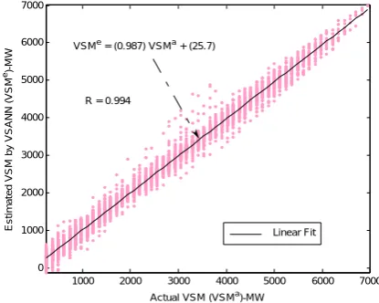
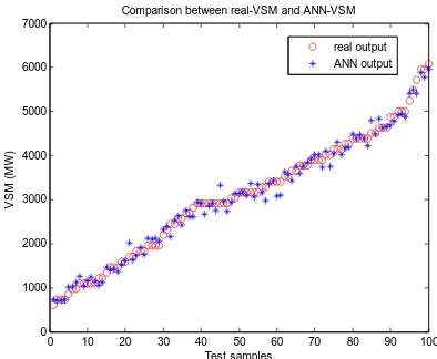
In addition to training, validating and testing errors, anotherpost-training analysis denoted as regression analysis has been performed relating VSANN response to the actual values to investigate the performance of the trained VSANN. For this purpose, linear regression between VSANN outputs and exact values is used to determine the accuracy of VSANN. In Fig. 7, the outputs of VSANN are plotted versus the exact values, while its slope and correlation coefficient are about 0.987 and 0.994 respectively which are very close to 1 indicating good performance of VSANN. Fig. 8 shows the estimated VSM by VSANN compared to the exact
values for 100 samples randomly selected for testing VSANN. The normalized error between exact and estimated values of VSM lies in the range of -0.17 to 0.14.
Fig. 5 New England 39-bus test power system.
Fig. 6 Trend of errors corresponding to training, validation
and testing in 34 epochs of training.
Fig. 7 Post regression analysis on TRAINLM.
0 5 10 15 20 25 30 35 0
0.5 1 1.5 2 2.5 3 3.5 4 4.5
Epoch
S
q
uar
ed E
rr
o
r
Training Validation Test
1000 2000 3000 4000 5000 6000 7000 0
1000 2000 3000 4000 5000 6000 7000
Actual VSM (VSMa)-MW
Es
ti
m
a
te
d
VSM
b
y
V
S
A
N
N
(
V
SM
e
)-M
W
R = 0.994
Linear Fit VSMe = (0.987) VSMa + (25.7)
Fig. 8 Comparison between exact VSM and ANN output.
Table 1 Characteristics of the trained VSANN.
Training
patterns Validation patterns patterns Test neurons Hidden
Training time (sec.)
3081 1026 6162 30 64.35
After training and testing VSANN, it is used in the working mode of the proposed algorithm shown in Fig. 1. In this mode, for any given operating point of power system by synchronous measurement of bus voltages, voltage magnitudes and phase angles are extracted as input data for estimating VSM by VSANN. If the estimated VSM is less than the desired voltage stability margin VSM*, then by means of sensitivity analysis the most effective bus will be selected for reactive power compensation. At each step of compensation, new voltage profile and VSM are evaluated. This process is carried out until VSM reaches VSM*.
As a case study, for an operating point with load level 7559.8 MW, the value of β in Eq. (13) is taken as 0.20 and two scenarios are studied in which all network buses are supposed to be equipped with 200 and 100 MVAr reactive power resources respectively. Tables 2 shows the result of compensation for the first scenario in which VSM has increased from 905.8 MW to 1463.2 MW through 28 steps of compensation with total 1400 MVAr compensation. Tables 3 shows the result of compensation for the second scenario. Figs. 9 and 10
Table 2 Results of reactive power compensation for scenario 1.
Sc.
No. (MW) PL0
Before
Compensation After Compensation Most
Effective Buses
Injected Reactive
Power (MVAr) VSM
By VSANN
(MW)
VSM by C.P.F. (MW)
VSM By VSANN
(MW)
VSM By C.P.F. (MW)
1 7559.8 905.8 853.52 1525.3 1463.2
3 150 4 100 8 50 12 50 15 150 16 200 18 200 21 200 24 200 27 100 Σ 1400
Table 3 Results of reactive power compensation for scenario 2.
Sc. No.
PL0 (MW)
Before
Compensation Compensation After Most
Effective Buses
Injected Reactive
Power (MVAr) VSM
By VSANN
(MW)
VSM by C.P.F. (MW)
VSM By VSANN
(MW)
VSM By C.P.F. (MW)
2 7559.8 905.8 853.52 1160.9 1219.3
3 100 4 100 8 50 12 50 18 100 21 100 24 100 26 100 27 100 Σ 800
0 10 20 30 40 50 60 70 80 90 100
0 1000 2000 3000 4000 5000 6000 7000
Test samples
VSM
(
M
W
)
Comparison between real-VSM and ANN-VSM
real output ANN output
Fig. 9 Voltage profiles before and after compensation-scenario 1.
Fig. 10 Voltage profiles before and after
compensation-scenario 2.
show voltage profiles before and after compensation through several steps of improvement for scenarios 1 and 2 respectively.
By comparing scenario 1 with 2, it can be deduced that smaller size of compensation leading to the choice of less efficient place for reactive power injection has resulted in less improvement for VSM. As it can be seen, after compensation at the most effective buses, voltage profile is moved upwards and corresponding VSM is improved. It is worth noting that the proposed approach is aimed to be a simple and fast algorithm for improving VSM by reactive power compensation rather than optimization.
7 Conclusion
In this paper, a new algorithm based on voltage profile and neural network application is proposed for fast estimating and enhancing voltage stability margin. In this approach, network voltage profile consisting of both phase and magnitude of bus voltages which are
measured synchronously by PMU constitutes the input pattern for VSANN. The most interesting feature of the neural network application used in this paper is its ability for sensitivity analysis of VSM with respect to bus voltages and reactive power compensation. Network voltage profile is a robust operating variable which contains the effect of load-generation pattern, network topology and reactive power compensation with no dependency on a specific topology of the network. In order to increase the efficiency of training process of VSANN, principle component analysis has been used as feature reduction for extracting more dominant feature of voltage profile. The main advantage of the proposed approach is its ability for direct estimation of VSM from bus voltages at any moment so that any change in network topology due to line outage has no effect on VSANN performance. The simulation results demonstrate the effectiveness and suitability of the proposed approach for fast evaluating and enhancing voltage stability in an online environment.
References
[1] Assis T. M. L., Nunes A. R. and Falcao D. M., “Mid and long-term voltage stability assessmnt using neural networks and quasi-steady-state simulation”, Power Engineering, 2007 Large Engineering Systems Conference, pp. 213-217, Oct. 2007.
[2] Amjady N. and Esmaili M., “Improving voltage security assessment and ranking vulnerable buses with consideration of power system limits”, Electrical Power and Energy Systems, Vol. 25, No. 9, pp. 705-715, 2003.
[3] Taylor C. W., Power system voltage stability, New York: McGraw-Hill; 1994.
[4] CIGRE Task Force 38-02-10. “Modeling of voltage collapse including dynamic phenomena”, 1993.
[5] Verbi G. and Gubina F., “A novel scheme of local protection against voltage collapse based on the apparent-power losses”, Electrical Power and Energy Systems, Vol. 26, No. 5, pp. 341-347, 2004.
[6] Tamura Y., Mori H. and Iwamoto S., “Relationship between voltage instability and multiple load flow solutions in electric power systems”, IEEE Transactions on Power Apparatus and Systems, Vol. 102, No. 5, pp. 1115-1125, May 1983.
[7] Kessel P. and Glavitsch H., “Estimating the voltage stability of a power system”, IEEE Transactions on Power Systems, Vol. 1, No. 3, pp. 346-354, July 1986.
0 5 10 15 20 25 30 35 40 0.8
0.85 0.9 0.95 1 1.05 1.1
Bus number
V
o
lt
age (p.
u
.)
Before compensation - VSM = 905.8103 MW After compensation - VSM = 1525.2983 MW
0 5 10 15 20 25 30 35 40 0.8
0.85 0.9 0.95 1 1.05 1.1
Bus number
V
o
lt
age (
p
.u
.)
Before compensation - VSM = 905.8103 MW After compensation - VSM = 1160.8865 MW
[8] Sharm the Ap Predic Transm Chicag [9] Caniza V. H., detecti Trans. 1441-1 [10] Ajjarap stabilit 1, pp. [11] Lof
P-Stabili IEEE T 326-33 [12] Ajjarap power stabilit No. 1, [13] Gao B Stabili IEEE 4, pp. [14] Löf P. “Fast IEEE No. 1, [15] Zhao look-a securit Energy 2004. [16] Wiszn Stabili Shedd 22, No [17] Cai L
Voltag and R Appro Lausan [18] Liu H.
Fast V Adapti System 2000. [19] Suthar ANN Assess System [20] Wan H
networ
ma C. and Gan pplicability of ction of V
mission and go, pp. 1-7, A ares C. A., De , “Compariso ion of proxim on Power 1450, August pu V. and Lee ty”, IEEE Tra 115-125, Febr -A, Anderson ity indices of Trans. on Pow 35, Feb. 1993
pu V. and C flow: A to ty analysis”, I
pp. 416-423, B., Morison G ity Evaluatio Transaction o 1529-1542, N . A., Smed T. calculation o Transactions pp. 54-64, Fe J., Chiang H ahead load m
ty Assessme y Systems, V niewski A., ity Margin ing”, IEEE Tr o. 3, pp. 1367-. J1367-. and Erlic ge Stability An Reactive Pow oach”, IEEE
nn, July 2007. ., Bose A. and Voltage Securi
ive Bounding ms, Vol. 15, N r B. and Bal
Based Metho sment”, IEE ms, Toki Mess H. B. and Ek rk based con
nness M. G., “D f using Modal
Voltage St d Distributio
pril, 2008. eSouza A. C. on of perform mity to voltage system, Vol. 1996. e B., “Bibliog ans. Power Sy
ruary 1998. n G. and Hill f the stressed wer Systems, V
.
Christy C., “T ool for stea IEEE Trans. o
Feb. 1992. G. K. and Kun
on Using M on Power Syst November 199 ., Anderson G of a voltage s on Power S ebruary 1992. H.-D. and Li margin estima ent”, Electric Vol. 26, No.
“New Crite for the Pu Trans. on Pow -1371, July 20 ch L., “Powe nalysis Consi wer Controls Power Tech . d Venkatasub ity Assessmen g”, IEEE Tr No. 3, pp. 11
lasubramanian d for Online V EE Conferen
e, Nov. 2007. kwue A. O., “ ntingency rank
Determination l Analysis for tability”, IE on Conferen Z. and Quint mance indices
e collapse”, IE 11, No. 3,
graphy on volt yst., Vol. 13, N l D. J., “Volt
power syste Vol. 8, No. 1,
The continuat dy-state volt on PWRS, Vol ndur P., “Volt Modal Analys tems, Vol. 7, N 92.
G. and Hill D stability inde Systems, Vol i H., “Enhan ation for volt cal Power a
6 ,pp. 431-4
eria of Volt urpose of L wer Pelivery, V
007.
er System St idering all Act
-Singular Va h, pp. 367-3 bramanian V.,
nt Method Us rans. on Pow
37-1141, Aug
n R., “A No Voltage Stabi nce on Pow
. “Artificial neu king method n of the EEE nce, tana for EEE pp. tage No. tage m”, pp. tion tage l. 7, tage sis”, No. . J., ex”, . 7, nced tage and 438, tage Load Vol. tatic tive alue 373, “A sing wer gust ovel ility wer ural for [21 [22 [23 Ele (PW Cen dyn app pro Pow to t boa dyn des voltage co Systems,V 1] Jolliffe I.
York: Spr 2] Aghamoh Dehghani rescheduli network Systems March 20 3] Tetko I.
“Neural overfitting Comput. S
ectrical Engine WUT), Tehran,
nter (IDRC). H namics and co plication in pow
ofessor in the wer and Water the ministry of ard in Iran. Hi namics and co sign, energy eco
ollapse”, Elec Vol. 22, pp. 34
T., Principal ringer-Verlag, hammadi M.
F., “Dynam ing using stab
as a preven Conference 09.
V., Livingsto network stad g and overt Sci., Vol. 35, N
Mohamma
received hi Univ. of T 1980, M.S (University U.K. in 19 Tohoku U electrical e assistant pr eering of Powe
Iran. He is he His research in ntrol, voltage wer system dyna
Seyed Sina
1985, He re Azad Univ. has joint University student sinc area voltag power syste Mohammad received his Univ. of Te M.Sc. degree Tech., Tehran from UMIST Manchester, U engineering. Department o Univ. of Tech energy and hea is research int ontrol, restructu onomics. ctrical Power 49-354, 2000. Component A , 1986. R., Magha mic security bility sensitivi ntive tool”, I
and Exposit one D. J. and dies. 1. Co training”, J. No. 5, pp. 826
d Reza Agh
is B.Sc. degre Technology Te Sc. degree f of Manchester 985 and Ph.D University in
engineering. H ofessor in the er an Water U
ad of Iran Dyn nterests include
stability and n amic.
Hashemi was eceived his B.S ., Aliabad, Iran
with Power of Technolo ce 2007. He has ge stability an em dynamics.
Sadegh
B.Sc. degree ech., Tehran, e from AmirK n, in 1988 and T (University o
U.K. in 1997, a He is curre of Electrical E h., Tehran, Iran
ad of the electri terests include
uring and elec
r and Energy Analysis, New ami A. and y constrained ties by neural IEEE Power tion, pp.1-7, d Luik A. I., omparison of Chem. Inf. 6-833, 1995.
hamohammadi
ee from Sharif ehran, Iran in from UMIST r), Manchester, . degree from 1995, all in He is currently Department of Univ. of Tech. namic Research power system neural network
born in Iran in Sc. degree from n in 2007. He r and Water gy as M.Sc. s worked on the nd control of
Ghazizadeh
e from Sharif Iran in 1982, Kabir Univ. of d Ph.D. degree of Manchester), all in electrical ently assistant Engineering of n. He is advisor icity regulatory power system ctricity market y w d d l r , , f f i f n T , m n y f . h m k n m e r . e f h f , f e , l t f r y m t