M
M
O
O
D
D
I
I
F
F
I
I
E
E
D
D
F
F
A
A
C
C
T
T
O
O
R
R
-
-
T
T
Y
Y
P
P
E
E
E
E
S
S
T
T
I
I
M
M
A
A
T
T
O
O
R
R
S
S
W
W
I
I
T
T
H
H
T
T
W
W
O
O
A
A
U
U
X
X
I
I
L
L
I
I
A
A
R
R
Y
Y
V
V
A
A
R
R
I
I
A
A
B
B
L
L
E
E
S
S
U
U
N
N
D
D
E
E
R
R
T
T
W
W
O
O
-
-
P
P
H
H
A
A
S
S
E
E
S
S
A
A
M
M
P
P
L
L
I
I
N
N
G
G
A
A
.
.
A
A
u
u
d
d
u
u
11,
,
A
A
.
.
A
A
.
.
A
A
d
d
e
e
w
w
a
a
r
r
a
a
22 1Department of Mathematics, Usmanu Danfodiyo University, P.M.B. 2346, Sokoto, Nigeria
2
Department of Statistics, University of Ilorin, P.M.B 1515, Ilorin, Kwara State, Nigeria Corresponding author: A. Audu, [email protected]
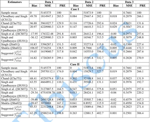
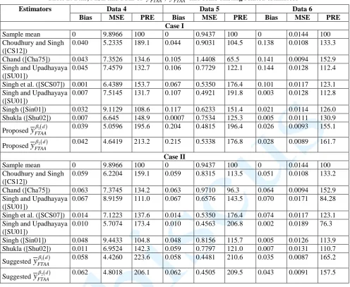
ABSTRACT: In this paper, two modified factor-type estimators with two auxiliary variables for population mean have been suggested. Bias and MSE of the suggested estimators have been derived up to first order approximation using Tailor’s series expansion and the conditions for their efficiency over some existing estimators have been established theoretically. Empirical study was conducted using three dataset and the results revealed that the suggested estimators are more efficient.
KEYWORDS: Estimator, Auxiliary variable, Mean square error (MSE), Two-phase sampling.
1.1 INTRODUCTION
Use of known functions of auxiliary variables in improving the performance of estimators has been one of the major strategies that have received wide attention of several authors like Chand ([Cha75]), Singh ([Sin01]), Singh and Upadhayaya ([SU01]), Singh et al. ([SUC04, SCS07]), Khan et al. ([KSS12]), Choudhury and Singh ([CS12]) in sampling survey. According to Choudhury and Singh ([CS12]), if auxiliary variable
X
is strongly correlated with another variableZ
, the known information onZ
like coefficients of kurtosis, skewness and variation e.t.c. help in increasing the efficiency of estimators if they are judiciously utilized.Let be a population of size and be three real valued functions having
values on the unit of . Let , and be the population means of ,
and respectively with and as coefficients of variation of , and respectively. Notations:
A
d
1
d
2
,B
d
1
d
4
,C
d
2
d
3
d
4
,d
is an unknown positive real number to be estimated i.e d1
,
2,
3,
4A C
fB
A
fB
C
A
fB C
A
fB C
A
fB C
A
fB C
, P
3 1 2 4Shukla ([Shu02]) suggested a factor-type estimator for population mean under two-phase sampling as
11FTd
A C x fBx y y
A fB x Cx
(1.1)
The bias and MSE of
y
FTd under case I and II are respectively
23 4
FTd I xy x y x
Bias y
YP
C C
C
(1.2)
21 3 2 4 2
FTd II x xy x y
Bias y
YP
C
C C
(1.3)
2 2 2 22 3
2
3FTd I y x xy x y
MSE y
Y
C
P C
P
C C
(1.4)
2 2 2 22 4
2
2FTd II y x xy x y
MSE y
Y
C
P C
P
C C
(1.5)2.0 SUGGESTED ESTIMATORS
Motivated by the work of Choudhury and Singh ([CS12]), the following factor-type estimators are suggested
1
1 1 2
2
1 2 1
d z z
FTAA
z z
A C x fBx a Z b y y
A fB x Cx a z b
(2.1)
2
2 1 2 1
2
1 2 2
d z z
FTAA
z z
A C x fBx a z b
y y
A fB x Cx a z b
(2.2)
Where 0
11, 0
2 13.0 PROPERTIES OF THE PROPOSED FACTOR-TYPE ESTIMATORS
In this section, the theoretical biases and MSEs of the suggested estimators are derived up to first order approximation using Taylor’s series expansion.
In order to study the properties of the proposed estimators, we define the following error terms
2 2
/
,
1 1/
,
2 2/
,
1 1/
,
2 2/
y
y
Y
Y
xx
X
X
xx
X
X
zz
Z
Z
zz
Z
Z
, such that2
1,
11 ,
21 ,
11 ,
21
y x x z z
Under case I: When secondary sample is a subset of preliminary sample
S
2
S
1
1 1 1
2 2 2
1 1 2 2 2
2 1 1 2
2 2 1 2 1
2 2 2
1 1 1
2 2 2
2 2 2 2 2 2 2 2
2 1 1 2
2 2
2 1 1
2
1 , 1 , 1
1 , 1 , 1
0
, , ,
, ,
,
y x z
y x z
x z y x z
y y x x z z x x
z z y x xy y x y z yz y z
y x xy y x y
y Y x X z Z
y Y x X z Z
E E E E E
E C E C E C E C
E C E C C E C C
E C C E
2 1 1
1 2 1 2 2 1
2 2 1 2
2 1
2
1 1 1
2
2 1 1 2 3 2 1
1 2
,
, ,
1 1 1 1
, , , ,
z yz y z x z xz x z
x z xz x z x x x x z xz x z
x z xz x z z z z
C C E C C
E C C E C E C C
E C C E C
n N n N
(3.1)
Under case II: When secondary sample is a subset of population
S
2
N
1 1 1
2 2 2
1 1 2 2 2
2 1 1 2
2 2 2 2 2
1 1
1 1 1
2 2 2
2 2 2 2 2 2 2 2
2 1 1 2
2 2
2 2 2
1
1 , 1 , 1
1 , 1 , 1
0
, , ,
, , ,
,
y x z
y x z
x z y x z
y y x x z z x x
z z y x xy y x y z yz y z
x z xz x z x
y Y x X z Z
y Y x X z Z
E E E E E
E C E C E C E C
E C E C C E C C
E C C E
1 2
1 2
2 2 21
2 1
2 1
1 2
2
0
z xz x z
x z x x x z y x y z z z
C C
E E E E E E
3.1 Bias and MSE of the estimator 1 d
FTAA
y
The suggested factor-type estimator 1 d
FTAA
y
can be expressed in terms of error terms1, 2, 1
x x z
and
2
y
is
1
1
2 1 2 1 2 1
1
1 2 3 4
1 1 1 1
d
FTAA y x x x x z z
y Y
(3.3)Here the assumption is that in (3.3),
1 2
3 x 4 x
1
and1
1
z z
so that
1 2
1
3 4
1
x
x and
11
1 z z
are expandable.
Subtract
Y
for both side of (3.3) and using power series expansion, the simplification of (3.3) up to first order approximation is given by
1
2 1 1 2 1 1 1 2 1
1 2 1 2 2 1 2 1 2 2
1 1 2 2
1 1 1
2 2
3 4 3 4 1 4 2 3 1
1
2
2
d
FTAA y z z x x z z z x z z x z
x x x x z y z y x y x
y Y Y P P P
P P P P
(3.4)
Taking expectation of (3.4) and apply the results in (3.1), the bias of the suggested estimator 1 d
FTAA
y
under case I is obtained as
1
2
2 1
1
23 4 1 1
1
2
d
FTAA x xy x y z z z yz y z
I
Bias y
Y
PC
C C
C
C C
(3.5)Also, taking expectation of (3.4) and using results of (3.2), the bias of the suggested estimator to terms of ordern1 under case II is obtained as
1
2 2
2
3 3 2 4 1 3 1 1 / 2
d
FTAA x x yx z z z xz
II
Bias y Y
P C P C
C
C
PC (3.6)Square both sides of (3.4), taking expectation and using the results in (3.1), we obtain the MSE of the suggested estimator 1 d
FTAA
y
under case I as:
1
2 2 2
2
2 3 2 1 1 1 2
d
FTAA y x yx z z z yz
I
MSE y Y
C
C P P C
C
C (3.7)Also, square both sides of (3.4), taking expectation and using the results in (3.2), we obtain the MSE of the suggested estimator 1 d
FTAA
y
under case II as:
1
2 2 2
2
2 2 2 3 3 1 1 2
d
FTAA y x yx z z z xz
II
MSE y Y
C C P
P C
P
C
PC (3.8)Differentiate equation (3.7) partially with respect to P and equate to zero,
1
2 23 3
2
2
0
d
FTAA x xy x y
I
MSE y
Y
P C
C C
P
(3.9)31
opt yx
P
C
P
(3.10)
1
2 2
2
1 1
1
2 0
d
FTAA z z z xz
I
MSE y Y
C
C
(3.11)
1
/
11opt yz z
C
(3.12)Substituting the values of P31opt and 11opt in equation (3.7) and simplify, we obtain minimum mean square error of 1 d
FTAA
y
under case I as
1
2 2 2 2min 2 3 1
d
FTAA y xy yz
I
MSE
y
Y C
(3.13)In order to estimate unknown constant d in the estimator 1 d
FTAA
y
under case I, P Cyx and P
3 1are equated as
3 1 Cyx
(3.14)yx
fB C
C
A C
fB
(3.15)
3 2
1
8
9
5
5
23
26
4
4
22
24
0
u
d
fu
f
u
d
fu
f
u
d
fu
f
u
(3.16)where u Cyx
By solving (3.16), at most 3 zeros and of the polynomials for which (2.1) is optimal under case I will be obtained.
Also, differentiate equation (3.8) with respect to P and
1 and equate to zero, we obtain:
1
2 2
2 2
2 1 1
2
2
0
d
FTAA x yx x z z xz
II
MSE y
Y
C
P C
PC
C C
P
(3.17)2 2
2 1 1
2 4
x yx z z xz x
C C C C P
C
(3.18)
1
2 2
2
1 1
1
2 0
d
FTAA z z z xz
II
MSE y Y
C
PC
(3.19)
1 PCxz / z
(3.20)Solving P and
1 simultaneously, the optimum values of Pand
1 are
2
2
/
4 1 32opt
yx xz
P
C
P
(3.21)
2
12 2
4 1
xy xz opt
z xz
C C
(3.22)
Substituting the values of P32opt and 12
opt
in equation (3.8) and simplify, we obtain minimum mean square error of 1 d
FTAA
y
under case II as
1
2 2 2
2
min 2
1
/ 1
1/
2 1/
2d
FTAA y xy xz
II
MSE
y
Y
C
(3.23)In order to estimate unknown constant d in the estimator 1 d
FTAA
y
under case II,
2
2 yx / 4 1 xz
P C
2
3 1 2Cyx/ 4 1 xz
(3.24)
2
2 yx
/
4 1 xzfB C
C
A C
fB
(3.25)
3 2
1
8
9
5
5
23
26
4
4
22
24
0
t
d
ft
f
t
d
ft
f
t
d
ft
f
t
(3.26)where
2
2 yx/ 4 1 xz
t C
By solving (3.26), at most 3 zeros and of the polynomials for which (2.1) is optimal under case II will be obtained.
3.2 Bias and MSE of the estimator 2 d
FTAA
y
To the first degree of approximation, the suggested factor-type estimator 2 d
FTAA
y
can be expressed in terms of error terms1, 2, 1, 2
x x z z
and
2
y
as
2 2
2
2 1 2 1 2 1 2
1
1 2 3 4
1 1 1 1 1
d
FTAA y x x x x z z z z
y Y
(3.27)Here, we now assume that in (3.92),
1 2
3 x 4 x
1
,1
1
z z
and2
1
z z
so that
1 2
1
3 4
1
x
x
,
21
1 z z
and
22
1 z z
are expandable.
Expanding the right hand side of (3.27) up to second degree approximation and then subtract
Y
, we have,
2
2 2 1 2 2 1 2
2 1 1 2 1 2 2 1 2 1 2 2
1 2 1 2 1 2 1 2 2
2 2 2 2
2 2
2 2
2 3 4 4 3 2
2 2
2 2 2 2
2 2 2 2
1
2
1
2
d
FTAA y z z x x z z z x z
z x z x x x x z y z y x y x
z z z z z z z z z x z z y z
y
Y
Y
P
P
P
P
P
P
P
P
P
P
P
(3.28)
Taking expectation of equation (3.28) and apply the results in equation (3.1), the bias of the suggested estimator
2d
FTAA
y
when S2 S1 is obtained as
2 2 2 2 2
2 1 3 4 3 2
2 2 2 2 2 2 2 2 2
2 1 2
1
1
2
2
d
FTAA yz z yx x x z yz z
I
z z z z
Bias y
Y
PC C
PC C
PC
C C
C
C
(3.29)
Also, taking expectation of (3.28) and using results of (3.2), the bias of the suggested estimator 2 d
FTAA
y
to terms of ordern1 when S2 N is obtained is obtained as:
2
2
2
2 2 2
2
2 2 22 1 2 2
2 2 2 2
3 1 4 2 2 2 2
1 1
2 2
d
FTAA z z z z z xz z
II
x x x yx z yz z
Bias y Y C C P C C
P C P C P C C C C
Square both sides of (3.28), taking expectation and using the results in equation (3.1), we obtain the MSE of the suggested estimator 2 d
FTAA
y
under case I as:
2
2 2 2
2
2 3 2 3 2 1 2 2
d
FTAA y x yx z z z yz xz
I
MSE y Y
C
C P P C
C
C PC (3.31)Also, square both sides of (3.28), taking expectation and using the results in equation (3.2), we obtain the MSE of the suggested estimator 2 d
FTAA
y
under case II as:
2 2 2 2 2
2 2 1 2 2
2 2 2
2 2 2 1
2 2
2 2
d
FTAA y x yx z z z xz
II
z z z yz xz x
MSE y Y C C P P C C PC
C C PC P C
(3.32)
Differentiate equation (3.31) with respect to P and equate to zero,
2
2 23 3 3 2
2
2
2
0
d
FTAA x xy x y z xz x z
I
MSE y
Y
P C
C C
C C
P
(3.33)2
/
xy y z xz z x
P
C
C
C
(3.34)Differentiate equation (3.31) with respect to
2 and equate to zero,
2
2 23 2
2
2 2 2 0
d
FTAA z z z yz xz
I
MSE y Y
C
C PC
(3.35)
2
C
yzPC
xz/
z
(3.36)Solving P and
1 simultaneously, the optimum values of Pand
1 are
41/
optxy y xz z yz x xz z xz
P
C
C C
C
C C
P
(3.37)
2
/
21opt x yz xy y xz z x xz z xz
C C
C C
C
C C
(3.38)Substituting the values of P41opt and 21 opt
in equation (3.31) and simplify, we obtain minimum mean square error of 2 d
FTAA
y
under case I as
2
2 2
2 2
2
min 2 3
2
/ 1
d
FTAA y xy yz xy xz yz xz
I
MSE
y
Y C
(3.39)In order to estimate unknown constant d in the estimator 2 d
FTAA
y
under case I,
/
xy y xz z yz x xz z xz
P
C
C C
C
C C
and P
3 1 are equated as
3 1 xy
C
y xzC C
z yz/
C
x xzC C
z xz
(3.40)
/
xy y xz z yz x xz z xz
fB C
C
C C
C
C C
A C
fB
(3.41)
3 2
1
8
9
5
5
23
26
4
4
22
24
0
m
d
fm
f
m
d
fm
f
m
d
fm
f
m
(3.42)By solving (3.42), at most 3 zeros and of the polynomials for which (2.2) is optimal under case I will be obtained.
Also, differentiate equation (3.32) with respect to P and
2 and equate to zero, we obtain:
2
2 2
24 2 4 2
2
2
0
d
FTAA x yx z z xz
II
MSE y
Y
C
P
C
C C
P
(3.43)2 2
4 2 2
2 4
z z xz x yx x
C C C C P
C
(3.44)
2
2 2 2 2 23 2 3 2
2
2 2 2 0
d
FTAA z z z z xz z z xz
II
MSE y Y
C
P C C
C C
(3.45)
2 2
C
xz 4PC
xz/
4 z
(3.46)Solving P and
2 simultaneously, the optimum values of Pand
2 are2
42 2
/
41
opt
yz xz y xy x xz
P
C
C
(3.47)
2
22 2
4
1
yz yx xz opt
z xz
C
C C
(3.48)Substituting the values of P42opt and 22opt in equation (3.32) and simplify, we obtain minimum mean square error of 2 d
FTAA
y
under case II as
2 2 2
min 2 2 2 2 2 4
4 2
4 2 4 2 2 2 2 2 4
4
2 4
1 2 1
2 2 1 2
1
2
yz xz xy y d
FTAA y yz xz y
II
xz
yz yx xz
xy y xz xy y yz y z
xz xz y z yz xz xy
C
MSE y Y C C
C C C
C C C C
C C
(3.49)
In order to estimate unknown constant d in the estimator 2 d
FTAA
y
under case II, 22 yz xz y xy / 4 x 1 xz
P C C and P
3 1 are equated as 23 1 2 yz xz Cy xy / 4Cx 1 xz
(3.50)
2 2 yz xz y xy
/
4 x1
xzfB C
C
C
A C
fB
(3.51)
3 2
1
8
9
5
5
23
26
4
4
22
24
0
q
d
fq
f
q
d
fq
f
q
d
fq
f
q
(3.52)where 2
2 yz xz y xy / 4 x 1 xz
q C C
4.0 EFFICIENCY COMPARISONS
In this section, the efficiency of suggested estimators are compared theoretically with that of some existing estimators in the literature and the conditions for which the suggested estimators performed better have been established.
4.1 Efficiency of 1 d
FTAA
y
over some related estimators1. The efficiency of suggested estimator 1 d
FTAA
y
and estimatory
RP dc suggested by Choudhury and Singh ([CS12]) are compared as,
1
min min
0
dc d
RP FTAA
I I
MSE y
MSE y
(4.1)
2
2 2
3 1
2 2 2 2 2 2 2 2
2 2 2 2 3 1
3 1
0
x yx z yz
y y x yx z yz
x z
C C C C
Y C Y C C C C C
C C
2 0 yx yz
C C
xy z yz
x
C
C
(4.2)
min min
0
dc d
RP FTAA
II II
MSE y
MSE y
(4.3)
2 2 4 2 2 4
2 2
2 2 2 2
2 2 2 2 2 2 2
4 1 4 1
0
1 2
yx x yx x
y y
x z xz x z xz
C C
C C
Y
C
Y
C
C
C
C
C
C C
21
0
xz
C
z xz
x
C C
(4.4)2. The efficiency of suggested estimator 1 d
FTAA
y
and estimator t31 suggested by Chand ([Cha75]) are compared as,
1
31
0
d FTAA
I I
MSE t
MSE y
(4.5)
2 2 2 2
2 3 1
2 2 2 2
2 3 2 1 1
1 2
1 2
2
2
0
y x yx z yz
y x yx z z z yz
Y
C
C
C
C
C
Y
C
PC
P
C
C
C
Set
1Cyz /
z as obtained in section 3.12 2
2 3 1
2 3
xy y x yz y z
yx
x
C C C C
P C
C
1/2
2 2 2
3 xy y x 1 yz y z
/
3 x yxP
C
C
C
C
C
C
(4.6)3. The efficiency of suggested estimator 1 d
FTAA
1
32
0
d FTAA
I I
MSE t
MSE y
(4.7)
2 2 2 2
2 3 1
2 2 2 2
2 3 2 1 1
1 2 2
2 2 0
y x yx z yz
z z
y x yx z z z yz
Z Z
Y C C C C C
Z C Z C
Y C PC P C C C
Set
1Cyz /
z as obtained in section 3.12 2
3 1
2
2 3
xy y x yz y z
z yx
x
Z
C
C
C
C
Z
C
P C
C
2 1/22 2
3 xy y x 1 yz y z
/
z/
3 x yxP
C
C
C
ZC
Z
C
C
C
(4.8)4. The efficiency of suggested estimator 1 d
FTAA
y
and estimatort
33 suggested by Singh et. al ([SCS07]) are compared as,
1
33
0
d FTAA
I I
MSE t
MSE y
(4.9)
2 2 2 2
2 3 1
2 2 2 2
2 3 2 1 1
1 2 2
2 2 0
y x yx z yz
xz xz
y x yx z z z yz
Z Z
Y C C C C C
Z Z
Y C PC P C C C
Set
1Cyz /
z as obtained in section 3.12 2
3 1
2
2 3
xy y x yz y z
xz yx
x
Z
C
C
C
C
Z
P C
C
2 1/22 2
3 xy y x 1 yz y z
/
xz/
3 x yxP
C
C
C
ZC
Z
C
C
(4.10)5. The efficiency of suggested estimator 1 d
FTAA
y
and estimatort
34 suggested by Upadhayaya and Singh ([SU01]) are compared as,
1
34
0
d FTAA
I I
MSE t
MSE y
(4.11)
2 2 2 2
2 3 1
2 2
2 2 2 2
2 3 2 1 1
1 2 2
2 2 0
z z
y x yx z yz
z z z z
y x yx z z z yz
C Z C Z
Y C C C C C
C Z C Z
Y C PC P C C C
2 2 3 1 2 2 2 3 z
xy y x yz y z
z z
yx
x
C Z
C
C
C
C
C Z
P C
C
1/ 2 2 2 23 1 3
2
/
z
xy y x yz y z x yx
z z
C Z
P C C C C C C
C Z
(4.12)6. The efficiency of suggested estimator 1 d
FTAA
y
and estimatort
35 suggested by Singh ([Sin01]) are compared as,
1
35
0
d FTAA
I I
MSE t
MSE y
(4.13)
1 12 2 2 2
2 3 1
1 1
2 2 2 2
2 3 2 1 1
1 2 2
2 2 0
z z
y x yx z yz
z z
z z
y x yx z z z yz
Z Z
Y C C C C C
Z Z
Y C PC P C C C
Set
1Cyz /
z as obtained in section 3.1 2 2 1 3 1 2 1 2 3 z
xy y x yz y z
z z yx
x
Z
C
C
C
C
Z
P C
C
1/2 2 2 23 xy y x 1 yz y 1z z
/
1z z/
3 x yxP
C
C
C
ZC
Z
C
C
(4.14)4.2 Efficiency of 2 d
FTAA
y
over some related estimators1. The efficiency of suggested estimator 2 d
FTAA
y
and suggested estimator 1 dFTAA
y
are compared as,
1
2
min min
0
d d
FTAA FTAA
I I
MSE y
MSE y
(4.15)2 2
3
2 2 2 2
2 3 1 2 2
2
0
1
xy yz xy xz yz
y xy yz
xz
Y C
2 23 yz xy xz 1 xz 0
2
1/21 3
1
1
xy xz xz yz
2
1/ 21 3
/
1
1
yz xy xz xz
(4.16)
1
2
min min
0
d d
FTAA FTAA
II II
MSE y
MSE y
(4.17)
2 2 2
2 2 2
1 2 2 2 1 0
y y xz yz xy y xz xy y