ASSOCIATION RULE MINING BASED VIDEO CLASSIFIER WITH LATE ACCEPTANCE HILL CLIMBING APPROACH

AN INVENTORY MODEL FOR NON-INSTANTANEOUS

DETERIORATING ITEMS UNDER TWO LEVELS OF TRADE

CREDIT AND TIME VALUE OF MONEY

1_{HAO JIAQIN,} 2_{CHEN GUOLONG,} 1_{CHEN PANFENG,} 3_YAO

_YUNFEI,

4_{ZHANG YADONG}

1_{School of Mathematics and Statistics, Suzhou University, Suzhou, Anhui, 234000, China;} 2

College of information engineering Suzhou University, Suzhou, Anhui, 234000, China;

3_{School of Mathematics and Computational Science, Fuyang Normal College, Fuyang, Anhui,}

236029, China;

4_{College of Mathematics and Information Science, Guangxi University, Nanning, Guangxi, 530004, China.}

Email: [email protected] ; [email protected] ; [email protected] ; [email protected];

5

[email protected]

ABSTRACT

In this study, in order to investigate the influence of the time value of money strategy, an inventory system for non-instantaneous deteriorating items under two-level trade credit is considered by using the discounted cash-flows (DCF) approach. The purpose of this paper is to find the optimal replenishment policies for min-imizing the total present value of all future cash-flow cost for the retailer. Useful theorems to characterize the optimal solutions have been derived. Numerical examples are provided to demonstrate the results.

Keywords: Two Levels Of Trade Credit; Non-Instantaneous Deteriorating Items; Time Value Of Money;

Inventory Model

1. INTRODUCTION

In the real markets, to motivate retailer to in-crease their order qualities, the supplier often pro-vides a permissible delay in payment to the retail-ers. Furthermore, the retailers may offer their cus-tomers a permissible delay period when they re-ceived a trade credit by the supplier, that is two-level trade credit. Goyal [1] was the first to explore an EOQ model under permissible delay in payment. Huang [2] extended [1] to develop an EOQ model under the two-level trade credit. Chung [3] dis-cussed an inventory model that trade credit depend-ed on the ordering quantity. Mahata [4] investigatdepend-ed an EPQ model with deteriorating items, which as-sumed that the retailer offered the partial trade cred-it to his/her customers when he/she received the full trade credit by the supplier. Liao [5] established an EOQ model for deteriorating items with two-storage facilities where trade credit was linked to order quantity.

The inventory models above ignored the ef-fects of the time value of money. In practice, all cash outflows have different values at different points of time. Therefore, it is necessary to take the time value of money on the inventory policy into

consideration. Chung [6] analyzed an EOQ model for deteriorating items and talked about the time value of money; Chung [7] discussed the effect of trade credit depending on the order quantity by us-ing the DCF approach; Liao [8] extended the inven-tory model by considering the factors of two levels of trade credit, deterioration and time discounting.

In the above deteriorating items inventory lit-eratures assumed that the deterioration of the items in inventory starts from the instant of their arrival in stock. In fact, most goods would have a span of maintaining quality before they deteriorated. Ouyang [9] established an inventory model for non-instantaneous deteriorating items with permissible delay in payments.

In this paper, an inventory system for non-instantaneous deteriorating item is investigated un-der two levels of trade credit and time value of money. The method of finding the optimal cycle time is proposed. Sensitivity analysis of major pa-rameters is given to obtain some managerial in-sights.1

1_{Corresponding Author: YAO YUNFEI, School of}

ISSN: 1992-8645 www.jatit.org E-ISSN: 1817-3195

2. NOTATIONS AND ASSUMPTIONS

2.1 Notations

The following notations are used throughout this paper.

A the ordering cost one order;

c unit purchasing cost per item; p unit selling price per item p>c;

h holding cost per unit time excluding int

erest charges;

r the continuous rate of discount;

D demand rate per year;

Q the retailer’ order quantity per cycle; T the cycle time;

( )

PV T∞ the present value of all future cash-flow

cost.

2.2 Assumptions

The mathematical model in this paper is devel-oped under the following assumptions

(1) Time horizon is infinite, and the lead time is negligible;

(2) Replenishments are instantaneous, and shortage is not allowed;

(3)Tθis the length of time during which the product

has no deterioration. If T≤Tθ, then the product

is no deterioration; else, a constant θ(0< <θ 1) fraction of the on-hand inventory deteriorates per unit of time and there is no repair or re-placement of the deteriorated inventory; (4) WhenT≥M , the account is settled att=M and

the retailer would pay for the interest charges on items in stock with rate Ip(per $ per year) dur-ing the interval

[

M T,

]

; whenT<M, the account is also settled att=M and the retailer does not need to pay any interest charge of items in stock during the whole cycle;

(5) The retailer can accumulate revenue and earn interest after his/her customer paying for the amount of purchasing cost to the retailer till the end of the trade credit period offered by the supplier. That is, the retailer can accumulate revenue and earn interest during the period

NtoMwith rate I_e(per $ per year) under the condition of trade credit; meanwhile the fixed credit period offered by the supplier to the re-tailer is not less to his/her customers, i.e.

0≤N≤M.

(7) ForT>Tθ, I t1

( )

denotes the level of inventory at

timet∈

(

0,Tθ

)

; I2

( )

t denotes the inventory level

at timet∈

[

T T_θ,

]

; I t

( )

denotes the level of in-ventory at timet∈

(

0,T

]

.

(8) By convenience, we Let

(

)

0

rM rN rM

e

rce− + −h pI e− −e− ≥ .

3 . MATHEMATICAL MODEL

Based on the assumptions above, when

0< ≤T Tθ , the items are depleted in the

inter-val

(

0,T

]

due to the effect of demand. At timet=T, the inventory level reaches zero. Thus, the invento-ry level can be described by the following differen-tial equation

' ( )

I t = −D, 0≤ ≤t TandT<Tθ,I T( )=0.

The solution to the equation is

( )

(

)

I t =D T−t , 0≤ ≤t TandT<Tθ.

In this case, the retailer’s order size per bicycle

(0)

Q=I =DT.

WhenT>T_θ, ift∈

(

0,T_θ

]

, then the level of in-ventory will decrease only owing to demand. Thus, the inventory level, I t₁

( )

, is given by the

differen-tial equation

' 1( )

I t = −D, 0≤ ≤t Tθ, I1(0)=Q.

The solution to the equation is

( )

1

I t = −Q Dt (1)

At the intervalt∈

(

T T_θ,

]

, the inventory level depletes to zero due to the effect of demand as well as deterioration. Hence, the inventory level,I₂

( )

t ,

is given by

( )

'

2( ) 2

I t = − −D θI T , Tθ≤ ≤t T, I T2( )=0. (2)

The solution to the equation is

( )

( )

2 1

T t

I t =D e_ θ − − _ θ , Tθ ≤ ≤t T. (3)

Considering the continuity ofI t

( )

at timet=Tθ,

i.e.

( )

( )

1 2

I T_θ =I T_θ .

Which implies that

( )

1

T T

Q DT D eθ θ

θ  −  θ

= + _ − _ .

Thus, we obtain

( )

(

)

( )

1 1

T T

I T D T t D eθ θ

θ  −  θ

= − + _ − _ .

( )

PV∞ T consists of the following elements (1) The present value of order cost

(

1 rT

)

O

V =A −e− ; (2) The present value of holding cost excluding interest charges.

When0< ≤T Tθ,

(

)

2

(

)

1 1

rT rT

H

V =hD e− +rT− _r −e− _;

(

) (

)

( ) 1 1 1 1 1 ; rT H rT

T T rT rT

hD

V e rT

r

r e

e e e

r r θ θ θ θ θ θ θ

θ θ θ

− − − − −  = _ + − − −     +  − ₊ +  +    

(3) The present value of purchasing cost. When0< ≤T Tθ,

(

1

)

rM rT

C

V =cDTe− −e− ;

WhenT>Tθ,

( )

(

)

1 1

T T

rM rT

C

V cDe T eθ θ e

θ

θ − θ

− _{  } − _

= _ + − _{ } − _.

(4) The present values of interest charged. WhenM ≤ ≤T T_θ,

(

)

2

(

)

1 1

rM rT rT

IP p

V =cI D e_ − rT−rM− +e− _{ } r −e− _;

WhenM ≤Tθ≤T,

(

)

(

)

( ) 1 1 1 1 ;

p rM rT

IP rT rT rM rT T T rM cI D

V e rT rM e

r

r e

e e e

e e r r θ θ θ θ θ

θ θ θ θ

− − − − − − − −    = _{ } − − + _ −      − + _ − _+ _ + _{+ }   

WhenTθ ≤M≤T,

(

)

(

)

( )

(

)

1

.

T r M p

IP rT

rT rM

cI D

V re

r r e

e r e

θ θ θ θ θ θ − + − − −  = _ + −  + − + _

(5) The present values of interest earned. When0< ≤T N,

(

rN rM

) (

1 rT

)

;

IE e

V = pI DT e− −e− _r −e− _

WhenN≤ ≤T M,

(

)

(

)

2 1 ;

1

rN rM rT

e

IE rT

pI D

V rN e rTe e

r e

− − −

−  

= _ + − − _

−

WhenM≤T,

(

)

(

)

(

)

2 1 1 .

1

rN rM

e

IE rT

pI D

V rN e rM e

r e

− −

−  

= _ + − + _

−

From the arguments above,PV T∞( )can be

ex-pressed as

( ) O H C IP IE

PV∞ T =V +V +V +V −V . Three situations can be set as

0<Tθ≤N; N≤Tθ ≤M; M ≤Tθ.

When0<T_θ≤N, PV T∞( )is given by

( )

( )

( )

( )

( )

11 12 13 14

, 0 ,

, ,

, ,

, ,

PV T T T

PV T T T N

PV T

PV T N T M

PV T M T

θ

θ

∞

 < ≤

 _{≤ ≤}  =  _{≤ ≤}   _≤  where

( )

(

)

(

)

11 2 1 1 1 ; rT rT

rM rN rM

e

hD

PV T A e

e r

DT

rce h pI e e

r − − − − −  = _ + − −     + _ + − − _ 

( )

( )

(

)

(

)

12 1 1 ; rT T T rT rN rM e DF hDe

PV T E e

e r r

D

pI T e e

r θ θ θ θ − − − − −  = ₋  + + ₊   − − _

( )

( )

(

)

(

)

13 2 1 1 1 ; rT T T rT

rN rM rT

e

DF hDe

PV T E e

e r r

pI D

rN e rTe e

r θ θ θ θ − − − − − −  = _ + + − _ +    − _ + − − _

( )

( )

(

)

( )

(

)

(

)

(

)

14 2 1 1 1

1 1 .

rT T T

rT

rT rM

T r M p

rN rM

e

D hDe

PV T E Fe

e r r

cI D e e

e

r r r r

pI D

rN e rM e

r θ θ θ θ θ θ θ

θ θ θ

− − − − − − + − −  = ₋  + + ₊    +  ₊ + ₊ −         − _ + − + _

(

)

(

)

2 1 1 ; rM rT c

E A De T

h

D e rT r

r θ θ θ θ θ θ θ − − = + −   + _ + − − _

(

)

rT

(

)

.

rM

F=ce− +hθ+r −θe− θ r θ+ r

 

 

SincePV11

( )

Tθ =PV12

( )

Tθ , PV12

( )

N =PV13

( )

N

andPV₁₃

( )

M =PV₁₄

( )

M , moreoverPV T∞( )is

contin-uous and well-defined.

WhenN≤Tθ≤M, PV T∞( )is given by

( )

( )

( )

( )

( )

21 22 23 24

, 0 ,

, ,

, ,

, ,

PV T T N

PV T N T T

PV T

PV T T T M

PV T M T

θ

θ

∞

 < ≤

 _{≤ ≤}  =  _{≤ ≤}   _≤  where

( )

( )

21 11 ;

PV T =PV T PV₂₃

( )

T =PV₁₃

( )

T ;

( )

( )

24 14 ;

PV T =PV T

( )

(

)

(

)

(

)

22 2 2

2 1 1 1 1 . rN e rT

rM rM rT

e e

hD pI D

PV T A rN e

e r r

D

DT rce h pI e e h pI

r r − − − − −  = _ − − + −   + + + + + _

SincePV₂₁

( )

N =PV₂₂

( )

N , PV₂₂

( )

T_θ =PV₂₃

( )

T_θ and

( )

( )

23 24

PV M =PV M , and PV T∞( )is continuous and

well-defined.

ISSN: 1992-8645 www.jatit.org E-ISSN: 1817-3195

( )

( )

( )

( )

( )

31

32

33

34

, 0 ,

, ,

, ,

, ,

PV T T N

PV T N T M

PV T

PV T M T T

PV T T T

θ

θ

∞

 < ≤

 _{≤ ≤}



=  _{≤ ≤}



 _≤



where

( )

( )

31 11 ;

PV T =PV T PV32

( )

T =PV22

( )

T ;

( )

(

)

(

)

(

)

(

)

(

)

33 2

2

2 1

1 1

1 1

1 1 ;

p rT

rM rM rT

p p

rN rM

e

D

PV T A h cI rM

e r

DT rce h cI e h cI e

r r

pI D

rN e rM e

r −

− − −

− −

 _{ }

= ₋  − _ + + _



+ + + + +



 

− _ + − + _

( )

( )

(

)

(

)

( )

(

)

(

)

(

)

34

2

2 1 1

1

1 1

1 1 .

rT T T

rT

p rM rT rM

T T

p rM rT p rT

rN rM

e

D hDe

PV T E Fe

e r r

cI D

e rT rM e re

r

cI cI D

De e e e

r r r r

pI D

rN e rM e

r

θ

θ

θ θ

θ

θ

θ

θ θ

θ θ

θ

θ θ θ

− −

−

−

− −

− − − −

− −



= _ + +

− _ +

 

+ _ − − + − _

 

+ _ − _+

+ +

 



 

− _ + − + _

SincePV31

( )

N =PV32

( )

N , PV32

( )

M =PV33

( )

M and

( )

( )

33 34

PV Tθ =PV Tθ , and PV T∞( ) is continuous and

well-defined.

4. THEORETICAL RESULTS

Lemma 1. Let *

x denote the minimizing value ofF x

( )

.

If f x

( )

is continuous and increasing on

[ ]

a b, , and '

( )

( )

rx

(

1 rx

)

2

F x = f x e− −e− .

(a) iff a

( )

≥0, then * =

x a; (b) iff a

( )

< <0 f b

( )

,

then * ₀ =

x x , where x₀ is the unique solution of

( )

0

f x = on

[ ]

a b, ; (c) if f b

( )

≤0, then * = x b.

Theorem 1. When0<Tθ≤N , the optimal cycle

time *

T will be determined by the following steps. (a) if f₁₁

( )

T_θ ≥0 , f₁₂

( )

N ≥0 and f₁₃

( )

M ≥0 ,

then * * 11

T =T ; (b) if f₁₁

( )

T_θ <0 , f₁₂

( )

N ≥0 and

( )

13 0

f M ≥ , then * * 12

T =T ; (c) if f₁₁

( )

T_θ <0 ,

( )

12 0

f N < and f₁₃

( )

M ≥0 , then * * 13

T =T ; (d) if

( )

11 0

f T_θ < , f₁₂

( )

N <0 and f₁₃

( )

M <0 , then

* *

14

T =T .

Theorem 2. WhenN≤Tθ≤M , the optimal cycle

time *

T will be determined by the following steps.

(a) if f₂₁

( )

N ≥0, f₂₂

( )

T_θ ≥0and f₂₃

( )

M ≥0, then

* *

21

T =T ; (b) if f21

( )

N <0 , f22

( )

Tθ ≥0 and

( )

23 0

f M ≥ , then * * 22

T =T ; (c) if f21

( )

N <0 ,

( )

22 0

f T_θ < and f₂₃

( )

M ≥0, then * * 23

T =T ; (d) if

( )

21 0

f N < , f22

( )

Tθ <0 and f23

( )

M <0 , then

* *

24

T =T .

Theorem 3. When M<Tθ , the optimal cycle

time *

T will be determined by the following steps. (a) if f₃₁

( )

N ≥0, f₃₂

( )

M ≥0and f₃₃

( )

T_θ ≥0, then

* *

31

T =T ; (b) if f₃₁

( )

N <0 , f₃₂

( )

M ≥0 and

( )

33 0

f Tθ ≥ , then T*=T32* ; (c) if f31

( )

N <0 ,

( )

32 0

f M < and f₃₃

( )

T_θ ≥0, then * * 33

T =T ; (d) if

( )

31 0

f N < , f₃₂

( )

M <0andf T₇

( )

_θ <0, then * * 34

T =T .

Proof. See Appendix.

5. NUMERICAL EXAMPLES

To illustrate the results obtained in this paper, we provide the following numerical examples. LetA=350,c=15, p=17, Ip=0.15, Ie=0.1, h=0.5,

0.08,

θ= D=1000, M=0.5, N=0.3, r=0.08,

0.2.

Tθ =

Example: when Tθ=0.2 , (a) if A=10 , then

( )

11 0

f T_θ > , f₁₂

( )

N >0 and f₁₃

( )

M >0, according

to Theorem 1(a) * *

11 0.1107

T =T = and

( )

*

PV_∞ T

( )

*

11 11 178290

PV T

= = ; (b) if A=100 , then

( )

11 0

f Tθ < , f12

( )

N >0, f13

( )

M >0and according to

Theorem 1 (b) * *

12 0.2960

T =T = and

( )

*

( )

*

2 12 183560

PV_∞ T =PV T = ;

(c) if A=350, then f11

( )

Tθ <0 and f12

( )

N <0,

ac-cording to Theorem 1(c) * *

13 0.4453

T =T = and

( )

*

( )

*

13 13 192090

PV_∞ T =PV T = ; (d) if A=1000, then

( )

11 0

f T_θ < ,f₁₂

( )

N <0 and f₁₃

( )

M <0, according to

Theorem1(d) * *

14 0.6661

T =T = and

( )

*

PV_∞ T

( )

*

14 14 206340

PV T

= = .

When T_θ=0.4andT_θ =0.7, the theroem2 and 3 are illustrated.

Table 1. the impacts of change ofM andN on * T and

* ( ) PV T∞ .

M N PV_∞

( )

T* *

T

0.5 0.30 192090 0.4453

0.35 192850 0.4582

0.40 193700 0.4727

0.6 0.30 188550 0.4467

0.35 189310 0.4598

0.40 190150 0.4743

0.7 0.30 185040 0.4482

0.35 185800 0.4613

0.40 186640 0.4759

The following inferences can be made based on table1.

(1) When other parameters are fixed, it shows that

( )

*

PV∞ T increase when the value of N in-crease, and decrease when the value of M in-crease.

(2) When other parameters are fixed, it shows that *

T increase when the value of Mand N in-crease.

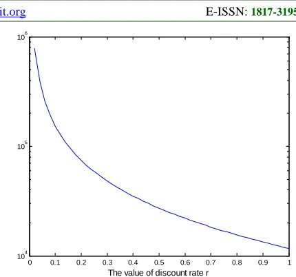
Figures 1-3 demonstrate the change of *

T , *

( ) PV T∞ ,

1

K and K2 when r is changed from(0,1

]

. T*and

*

PVare the value of the optimal cycle time and the value of optimal present value when r=1 ,

(

*

)

*

1 *

K = T −T T and

( )

*

( )

*

2 *

K =PV∞ T −PV PV∞ T .

0 0.1 0.2 0.3 0.4 0.5 0.6 0.7 0.8 0.9 1

0.25 0.3 0.35 0.4 0.45 0.5

[image:5.612.308.523.73.274.2]

The value of discount rate r

Fig. 1. The Impact Of Change OfrOn *

T .

0 0.1 0.2 0.3 0.4 0.5 0.6 0.7 0.8 0.9 1

104 105 106

The value of discount rate r

Fig. 2. The Impact Of Change OfrOn *

( ) PV T∞ .

0 0.1 0.2 0.3 0.4 0.5 0.6 0.7 0.8 0.9 1

0 0.1 0.2 0.3 0.4 0.5 0.6 0.7 0.8 0.9 1

The value of discount rate r

K1 K2

Fig. 3. The Impact Of Change OfrOnK1AndK2.

Figs. 1-3 give the following results: When rincreases, *

T ,

( )

*

PV∞ T , K1and K2

decreas-ing.

6. CONCLUSIONS

[image:5.612.97.299.461.645.2]

ISSN: 1992-8645 www.jatit.org E-ISSN: 1817-3195

situations under two-level trade credit and time value of money, such as the demand depending on the selling price, limited storage space, etc.

ACKNOWLEDGMENT

This work was supported by the national

specific Subject of the Ministry of Education

and the Ministry of Finance of the PRC

(TS11496), the National Natural Science

Foundation of China (No. 11226200) , and the

national statistics scientific research project

(2011LY094), and the

key Project of natural

science of universities in Anhui Province (No. 2005Kj023ZD).

REFRENCES:

[1]. S.K. Goyal, “Economic order quantity under conditions of permissible delay in payments”,

Journal of the Operational Research Society, 36, 1985, pp. 335–338.

[2]. Y.F. Huang, “Optimal retailer’s ordering poli-cies in the EOQ model under trade cre dit fi-nancing”, Journal of the Operational Research Society, 54, 2003, pp. 1011–1015.

[3]. K.J. Chung, “The simplified solution proce-dures for the optimal replenishment decisions under two levels of trade credit policy depend-ing on the order quantity in a supply chain sys-tem”. Expert Systems with Applications, 38, 2011, pp. 13482–13486.

[4]. G.C. Mahata, “An EPQ-based inventory model for exponentially deteriorating items under re-tailer partial trade credit policy in supply chain”, Expert Systems with Applications, 39, 2012, pp. 3537–3550.

[5]. J.J. Liao, K.N. Huang, and K.J. Chung, “Lot-sizing decisions for deteriorating items with two warehouses under an order-size-dependent trade credit”, International Journal of Produc-tion Economics, 137, 2012, pp. 102–115. [6]. K.J. Chung , and S.D. Lin, “The inventory

model for trade credit in economic ordering policies of deteriorating items in a supply chain system”, Applied Mathematical Modelling, 35, 2011, pp. 3111–3115.

[7]. K.J. Chung , and J.J. Liao, “The optimal order-ing policy of the EOQ model under trade credit depending on the ordering quantity from the DCF approach”, European Journal of Opera-tional Research, 196, 2009, pp. 563–568. [8]. J.J. Liao, and K.N. Huang, “An Inventory

Model for Deteriorating Items with Two Lev-els of Trade Credit Taking Account of Time

Discounting”, Acta Applicandae Mathemati-cae, 110, 2010, pp. 313–326.

Appendix. Proof: Taking derivative

ofPV Tij( )

(

i=1, 2,3;j=1, 2,3, 4

)

with respect toT, we obtain

( )

( )

(

)

' 2, 1 rT ij ij _rT

f T e

PV T e − − = − where ( ) ( )

(

) {

( )

11 (1 ) 11 1

1 ,

rT rT T rM

T rT

rT rN rM

e

f T r e PV T e D ce

pI

e e

h e e e

r r θ θ α α θ − − − − − − = − − + −  − _{ } + ₊ −  + − − _

( )

( )

(

)

( )

(

)

12 (1 ) 12 1

, T T rT rT rT rN rM e

f T r e PV T e D Fe

he pI e e r r θ θ θ − − − − −  = − − + − _  − − − _ + 

( )

( )

(

)

( )

(

)

13 (1 ) 13 1

, T T rT rT rT rT rM e

f T r e PV T e D Fe

he pI

D e e

r r θ θ θ − − − − −  = − − + − _  − − − _ + _

( )

( )

(

)

{

( ) ( )

(

)

14 (1 ) 14 1

1

,

T T

rT rT

T r M rT

p p

f T r e PV T e D Fe

cI e h cI e

r θ θ θ θ θ − − − + − = − − + −    + _{+ } − + _ 

( )

( )

(

)

(

)

(

)

22 22 1

(1 ) 1

1

,

rT rT rT

e

rM rM

e

f T r e PV T e D e h pI

r

rce h pI e

r − − − −  = − − + − _− +  + + + _

( )

(

)

(

)

(

)

( )

33 33 1 1 1

(1 ) ,

rT rM rM

p

rT rT

p

f T e D rce h cI e

r

e h cI r e PV T

r − − − −  = − _ + +  − + _− −

( )

(

)

( )

(

)

( )

(

) (

)

( )

34 34 1

(1 ) ,

rT T T

rT

p

T T p rM rT

rT

e

f T e D e F h cI

r

cI

e r e e

r r

r e PV T

θ θ θ θ θ θ θ θ θ − − − − − −  = −  − ₊ +     + _ + − _ + _ − −

( )

( )

23 13 ,

f T = f T f14

( )

T = f24

( )

T , f22

( )

T = f32

( )

T ,

( )

11 0

f = −rAand lim 14

( )

.

T→+∞f T = +∞ Tlim→+∞f34

( )

T = +∞.

Taking derivative off1i( )T

(

i=1, 2,3, 4

)

with

respect toT, we find that

( )

( )

( )

(

) (

)

' ' '

11 21 31

1 ,

T rM

rN rM rT e

f T f T f T

De rce h

pI e e e

θ − − − = =  = _ +  − − _ −

( )

(

)

(

)

( )

(

)

'

12 1 ,

T T

rT rN rM

e

f T ₌ e ₋ Dθ₊r Feθ −θ ₋pI e− ₋e− 

 

( )

( )

(

)

(

)

( )

' '

13 23

1 T T ,

rT rM

e

f T f T

e D θ r Feθ −θ pI De−

=   = − _ + + _

( )

( )

(

)

(

)

( ) ' ' 14 24

1 T r M ,

rT T

p

f T f T

e Deθ θ r Fe−θθ cI e− +θ

=   = − _ + + _

( )

( )

(

) (

)

' ' 22 32 1 ,

rT rM rM

e

f T f T

e D rce− h pI e−

=

= − + +

( )

(

) (

)

'

33 1 ,

rT rM

p

f T = e − D rce− + +h cI

( )

(

)

( )

₍

_){

(

) (

)

' 34 1 . T T rT

p rM rT

f T e De r F

cI

r e e

r r θ θ θ _θ θ θ θ − − − = − +    + _ + − _ + _

From assumption (6), we know that

( )

'

11 0,

f T ≥ f12'

( )

T ≥0,

( )

'

13 0,

f T ≥ f14'

( )

T ≥0 and