The Ads/CFT spectrum via Integrability based algorithms

integrability-based algorithms

Christian Marboe

School of Mathematics, Trinity College Dublin

College Green, Dublin 2, Ireland

Submitted to The University of Dublin for the degree of Doctor in Philosophy

Academic advisor: Dr. Dmytro Volin

I declare that this thesis has not been submitted as an exercise for a degree at this or any other university and it is entirely my own work.

I agree to deposit this thesis in the University’s open access institutional repository or allow the Library to do so on my behalf, subject to Irish Copyright Legislation and Trinity College Library conditions of use and acknowledgement.

The AdS/CFT correspondence has given rise to new tools that enable both perturbative and non-perturbative calculations of unseen precision in four-dimensional quantum field theories. The topic of this thesis is the spectral problem of the AdS5/CFT4correspondence in the planar limit, which from the point of view of the CFT, N = 4 super Yang-Mills theory, amounts to determining the spectrum of anomalous dimensions of single-trace operators.

There is substantial evidence that the spectral problem is integrable in the planar limit. This surprising asset makes the problem exactly solvable, and allows the application of sophisticated techniques to reformulate it. The Quantum Spectral Curve formulates the problem in terms of a relatively simple Riemann-Hilbert problem. To produce physical results from the Quantum Spectral Curve, one needs to solve it explicitly. There is one solution for each symmetry multiplet of single-trace operators. The main goal of this thesis is the development of efficient algorithms to find perturbative solutions for arbitrary multiplets. The two main steps of this process are, first, to find leading solutions and, second, to generate perturbative corrections.

To classify symmetry multiplets of single-trace operators, the relevant aspects of rep-resentation theory of non-compact super Lie algebras is revisited. It is argued that a generalisation of Young diagrams provides a convenient classification and leads to an in-tuitive way to count the multiplets.

The leading solution to the Quantum Spectral Curve is traditionally found by solving Bethe equations. These equations are hard to solve in practice, and the number of solutions exceeds the expectation from representation theory. To overcome these issues, a stronger criterion on the solutions is formulated, and an efficient algorithm to enforce this criterion is introduced. The result is a conceptually simple algorithm that is not only significantly more efficient than the solution of Bethe equations, but also yields exactly the expected number of solutions.

The perturbative corrections to the leading solutions are controlled by the analytic structure imposed by the Quantum Spectral Curve. Different strategies to recursively generate these corrections are discussed, and the ultimate approach is argued to be a con-cise algorithm to solve the Pµ-system for general states. This opens the door to a vast range of new spectral data, including 10-loop anomalous dimensions for a variety of mul-tiplets. This data is furthermore used to reconstruct the six- and seven-loop contributions to the anomalous dimension of twist-2 operators with arbitrary spin.

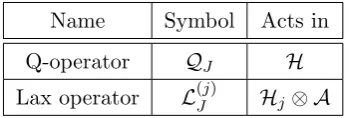
Finally, an attempt to apply the Quantum Spectral Curve on the operatorial level is initiated. In particular, a general strategy to evaluate matrix elements of Q-operators for non-compact super spin chains is outlined.

List of publications

The thesis is based on the author’s research presented in the publications

[1] Quantum spectral curve as a tool for a perturbative quantum field theory

with D. Volin,Nucl.Phys. B899 (2015) 810-847,[arXiv:1411.4758].

[2] Six-loop anomalous dimension of twist-two operators in planar N = 4

SYM theory

with D. Volin and V. Velizhanin,JHEP 1507 (2015) 084,[arXiv:1412.4762].

[3] Twist-2 at seven loops in planar N=4 SYM theory: Full result and ana-lytic properties

with V. Velizhanin,JHEP 1611 (2016) 013,[arXiv:1607.06047].

[4] Fast analytic solver of rational Bethe equations

with D. Volin,J.Phys. A50 (2017) no.20, 204002,[arXiv:1608.06504].

[5] The full spectrum of AdS5/CFT4 I: Representation theory and one-loop Q-system

with D. Volin,[arXiv:1701.03704].

[6] Evaluation of the operatorial Q-system for non-compact super spin chains

with R. Frassek and D. Meidinger,JHEP 1709 (2017) 018,[arXiv:1706.02320].

Furthermore, a substantial part of the thesis is based on yet unpublished work that will appear in

[7] The full spectrum of AdS5/CFT4 II

with D. Volin,work in progress.

Introduction 1

I The spectral problem in AdS/CFT integrability 7

1 Single-trace operators in N = 4 SYM 8

1.1 Representations of graded super Lie algebras . . . 8

1.2 Young diagrams. . . 14

1.3 Characters and counting . . . 20

1.4 The N = 4 SYM spectrum . . . 22

2 Spin chains and integrability 33 2.1 The Heisenberg spin chain and coordinate Bethe ansatz . . . 33

2.2 Algebraic Bethe ansatz. . . 38

2.3 Q-operators . . . 44

2.4 Generalisation to higher rank symmetry . . . 50

3 AdS/CFT integrability 55 3.1 Integrability in N = 4 super Yang-Mills theory . . . 55

3.2 Integrability in type IIB string theory . . . 57

3.3 The asymptotic Bethe ansatz . . . 59

3.4 The thermodynamic Bethe ansatz . . . 64

3.5 From TBA to QSC . . . 67

4 Quantum Spectral Curve 70 4.1 The Quantum Spectral Curve . . . 70

4.2 Important relations . . . 79

4.3 The QSC at weak coupling . . . 85

4.4 Applications and generalisations . . . 91

II The explicit spectrum 95

5 The 1-loop Q-system 96

5.1 Traditional methods . . . 97

5.2 Q-systems on compact Young diagrams . . . 100

5.3 Q-systems on non-compact Young diagrams . . . 107

5.4 Leading solution to the Quantum Spectral Curve . . . 112

6 Perturbative algorithms 119 6.1 Generalities . . . 119

6.2 Pµ-system for thesl(2) sector . . . 122

6.3 Solving the Q-system in general . . . 128

6.4 Solving the Pµ-system in general . . . 132

6.5 Results. . . 135

7 Twist-2 operators 144 7.1 Series of solutions and patterns in the data . . . 144

7.2 Twist-2 at six loops . . . 152

7.3 Twist-2 at seven loops . . . 154

8 QSC with Q-operators? 158 8.1 Evaluating Q-operators for non-compact super spin chains . . . 158

8.2 Q-operators in the Quantum Spectral Curve . . . 165

Conclusion 170 Acknowledgements 173 A Miscellanea 175 A.1 Quantum number dictionary . . . 175

A.2 Characters in practice . . . 176

A.3 Multiplet content of N = 4 SYM . . . 180

A.4 QSC-related technicalities . . . 183

A.5 The LLL-algorithm . . . 185

B Special functions 187 B.1 Zeta-values . . . 187

B.2 Harmonic and binomial sums . . . 190

B.3 Eta-functions . . . 193

B.4 Pochhammer, Gamma, Beta and Hypergeometric functions . . . 196

C.2 Evaluating auxiliary space traces . . . 201

Bibliography 203

Introduction

Quantum field theory is by far the most successful framework for describing the nature of elementary particles. The guiding principle for model building within this framework is symmetry. The fundamental objects in the theory, the fields, represent this symmetry choice. This starting point is however obscured by the quantum mechanical nature of the interactions between the fields. In consequence, quantum field theory is mainly a perturbative tool: we have to start from the limit of no interactions, and then gradually turn on the coupling. Many fundamental questions, such as the confining properties of quarks, cannot be described in this way. Furthermore, perturbative quantum field theory is an immensely complicated procedure. Not only do the combinatorics grow so rapidly that supercomputers quickly come to terms. One also has to go through the tedious mathematical procedures of regularisation and renormalisation for each individual process contributing to the result under study. In contrast, the results of these lengthy calculations often turn out to be strikingly simple. Sometimes just simple integer numbers. One naturally starts to wonder whether there is a simpler structure behind.

There exists a quantum field theory in four spacetime dimensions where such under-lying mathematical structures have been discovered. Again, symmetry was the guiding principle that led theoretical physicists towards it: the theory has the maximal amount of supersymmetry that can be put into a four-dimensional quantum field theory. The math-ematical structures appearing in this theory allow not only efficient perturbation theory, but also give rise to non-perturbative tools allowing explicit results at any interaction strength.

This thesis is a contribution to the effort of understanding the appearance and use of these structures. It is devoted to the use of a particular structure as a super-efficient perturbative tool. Before explaining the precise goals that are pursued, we take a brief look at the theory that is under investigation.

The remarkable features of

N

= 4

super Yang-Mills theory

N = 4 super Yang-Mills theory [8], or N = 4 SYM for short, is a theory with many particular properties. On one hand, these properties mean that the theory is certainly not

an adequate description of Nature, but on the other hand, they make the theory easier to analyse. It is of course important to ask to what degree the found structures have a generalisation in more realistic theories or if they are specific toN = 4 SYM. In this thesis we are not that ambitious: the goal is simply to demonstrate that there is something about this theory that is worth trying to generalise.

Yang-Mills theory is the type of quantum field theory on which the Standard Model

of particle physics is built. It is based on the invariance of physical observables under local transformations belonging to a Lie group, in our case SU(N). “N = 4” refers to the amount of supersymmetry, and this is the maximal amount in a four-dimensional theory with fields of spin no higher than one. This has profound consequences.

Superconformal symmetry

The field content in N = 4 SYM is six real scalars, four Weyl fermions, and a single gauge boson, all transforming in the adjoint representation of the SU(N) gauge group, and forming one big N = 4 supermultiplet. The Lagrangian of the theory is invariant under conformal transformations, which is not unusual. It is however unusual that the conformal invariance is not spoiled by quantum corrections. The single coupling constant appearing in the theory,gYM, is not subject to renormalisation, i.e. theβ-function is zero [9]. The generators of conformal symmetry combine with the supersymmetry generators to the larger superconformal algebra, which is isomorphic to the graded super Lie algebra

psu(2,2|4), including also the additional bosonic R-symmetry.

Correlation functions are the basic objects to study in quantum field theory, and conformal symmetry constrains the structure of these functions significantly, see e.g. [10]. The key object to study in a conformal field theory is the spectrum of the dilatation

operatorD, i.e. the generator of dilatations xµ→c xµ. This eigenproblem reads

DO(0) = ∆O(0), (1)

whereO(x) is a local operator and ∆ is itsconformal dimension. In general, all quantities in this equation are subject to quantum corrections and acquire a dependence on the coupling g. The coupling-dependent part of the conformal dimension is referred to as the

anomalous dimension γ,

∆(g) = ∆0+γ(g), (2)

where ∆0 ≡ ∆(0) is referred to as the classical dimension. The conformal dimensions completely determine two-point functions, which for scalar operators with suitable nor-malisation are given by

hOi(x1)Oj(x2)i=

δij |x₁−x2|2∆i

Introduction 3

Together with thestructure constantsCijk, the conformal dimensions also determine three-point functions to be

hOi(x1)Oj(x2)Ok(x3)i=

Cijk

|x₁−x2|∆1+∆2−∆3|x2−x3|∆2+∆3−∆1|x1−x3|∆1+∆3−∆2 . (4)

Higher-point functions are, in principle, also given by the conformal data {∆i, Cijk} through operator product expansions.

Importantly, as the anomalous part of the dilatation operator commutes with the gen-erators of the superconformal algebra, all opgen-erators related by symmetry transformations have the same anomalous dimension, see e.g. [11].

The AdS/CFT correspondence

According to the conjectured AdS/CFT correspondence [12],N = 4 SYM and type IIB su-perstring theory on AdS5×S5 are equivalent theories. In particular, local gauge-invariant operators inN = 4 SYM correspond to string states, and the conformal dimensions of the former are dual to the energies of the latter. The first hint of an equivalence is seen by matching the symmetries: the isometries of AdS5 and S5 fit with the bosonic subalgebras

su(2,2) and su(4) of the superconformal symmetry.

One of the reasons why the AdS/CFT correspondence is exciting is that in certain limits it relates strongly coupled gauge theory to weakly coupled string theory or simply supergravity. This opens the door to non-perturbative studies of quantum field theory.

Integrability in the planar limit

In this thesis, we will consider the AdS/CFT correspondence in the ’t Hooft limit where the coupling gYM is sent to zero, while the rank N of the SU(N) gauge group is sent to infinity. The product λ= g_YM2 N is kept finite. We will usually redefine this ’t Hooft

couplingby

g≡ √

λ

4π . (5)

The limit N → ∞ suppresses non-planar interactions, and it is thus called the planar

limit. In this limit, the theory displays yet another remarkable property: there is strong

evidence that at least certain aspects of the theory becomeintegrable. Integrability is the presence of an infinite set of conserved charges, and in some sense this makes the theory exactly solvable.

believed to encode the spectrum of anomalous dimensions at any value of the coupling:

theQuantum Spectral Curve [14,15].

The Quantum Spectral Curve as a perturbative tool

The Quantum Spectral Curve (QSC) is a unique discovery in the study of four-dimensional quantum field theories: it is a rather simple mathematical structure that can be solved to obtain explicit results at any value of the coupling. With such a framework at hand, we should understand how to exploit it – both to demonstrate its power, but also to test its scope and validity. The main goal of this thesis is to master this framework as a perturbative tool.

We first need to understand the objects under study: local gauge-invariant operators built by a single trace over fundamental fields. These objects have already been studied thoroughly in the literature, but we need to rephrase their classification in a language relevant for the QSC. Solving the QSC perturbatively has two main steps: finding the leading solution and perturbing around it. The problem of finding the leading solution is equivalent to solving Bethe equations for a certain type of spin chain. Again, the literature contains several approaches to doing this, but none which have the practical power that we are looking for. This thesis presents a new approach to this task, and the result is a method that is useful not only for the QSC, but for spin chains in more generality. Perturbative corrections can be generated through a recursive procedure repeating a small set of closed operations. However, the complexity of the appearing expressions grows rapidly, and the presented algorithms are the result of several cycles of implementation and optimisation. The final result is an automatisation of the procedure that gives access to a much wider range of explicit data than in previous studies.

Introduction 5

Structure of the thesis

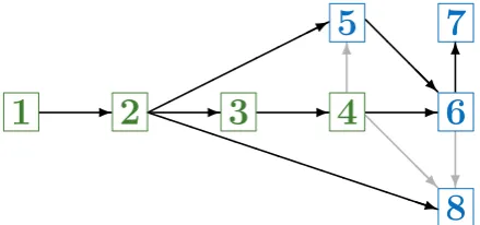
In an attempt to make a distinction between review and original work, the thesis has two main parts. The connection between the chapters is summarised in figure1.

Part I: The spectral problem in AdS/CFT integrability is mainly a review and contains four chapters:

1 Single-trace operators inN = 4 SYM revisits the representation theory relevant

for classifying symmetry multiplets of single-trace operators in N = 4 SYM. It contains a few new ideas, in particular the concept of extended Young diagrams, which have been presented in [5].

2 Spin chains and integrability introduces the key concepts of integrability –

co-ordinate and algebraic Bethe ansatz – in a simple setting, the Heisenberg spin chain. The generalisation to models with higher rank symmetry is briefly discussed.

3 AdS/CFT integrability gives a brief review of the appearance of integrability in

the spectral problem of the AdS/CFT correspondence. The basic ideas behind the techniques to bootstrap the spectrum by assuming integrability – the asymptotic and thermodynamic Bethe ansatz – are summarised.

4 Quantum Spectral Curve presents the QSC in an axiomatic form and discusses

all technical details that are needed for using it as a perturbative tool.

Part II: The explicit spectrum presents the original research on which the thesis is based, and it also contains four chapters:

5 The 1-loop Q-system is based on [4] and [5] and explains a new powerful method

to solve Bethe equations for rational spin chains, of which the leading solution to the QSC is a special example.

6 Perturbative algorithms is based on [1] and the yet unpublished work [7]. It

explains first a strategy to solve the QSC perturbatively for multiplets belonging

? 6

@ @

@ @ R

- - -

*

P P

P P

P P

P P

P P

P P

PPq @

@ @

@ R

6

1

2

3

4

5

6

7

to the sl(2) subsector and then a completely general algorithm, before presenting a sample of results.

7 Twist-2 operators is based on [2] and [3] and summarises how the produced data

can be used to reconstruct six- and seven-loop contributions to the analytically continued anomalous dimension for the infinite series of twist-2 operators.

8 QSC with Q-operators? is based on [6] and outlines a general strategy to evaluate

Part I

The spectral problem in AdS/CFT

integrability

Single-trace operators in

N

= 4

SYM

The goal of this thesis is to study anomalous dimension of local gauge-invariant operators made out of the fundamental fields in N = 4 SYM. The fields are all in the adjoint representation of theSU(N) gauge symmetry, but as we ensure gauge-invariance by tracing over the colour indices, the colour structure is completely absent in our treatment. The fields constitute a representation of the global symmetry of the theory, generated by the superconformal algebra, which is isomorphic to the graded super Lie algebra psu(2,2|4). Composite local operators with several field insertions can then be thought of as tensor products, and they will form more general irreducible representations of the symmetry. All operators within such a multiplet have the same anomalous dimension γ(g), and we can restrict our attention to single-trace operators, since they do not mix with operators containing multiple traces in the planar limit, see e.g. [11].

To classify the multiplets of single-trace operators, this chapter reviews the relevant aspects of representation theory of graded super Lie algebras before specialising to the case of N = 4 SYM. The goal is to find a convenient way to classify the multiplets and understand the multiplet content ofN = 4 SYM quantitatively.

1.1

Representations of graded super Lie algebras

In the following we will consider graded super Lie algebras that are real forms of gl(N+ M|K) and their unitary representations. The treatment will be informal, and the notation will not distinguish abstract Lie algebra generators from their realisation as explicit endo-morphisms of representation modules. Likewise, we will always understand the abstract Lie algebra bracket as an (anti-)commutator.

1.1. Representations of graded super Lie algebras 9

1.1.1 Definitions

Let us start by introducing the basic nomenclature. The generators,Emn, ofgl(N+M|K) satisfy the (anti-)commutation relation

EmnEkl−(−1)(pm+pn)(pk+pl)EklEmn = δnkEml−(−1)(pm+pn)(pk+pl)δmlEkn,(1.1)

wherem= 1, ..., N+M+K. We introduce two gradings, pm and cm, taking the values

m 1, ..., N N+1, ..., N+M N+M+1, ..., N+M+K

pm 0 0 1

cm 1 0 0 . (1.2)

The real formu(N, M|K) is obtained by imposing the conjugation property

E_mn† = (−1)cm+cn_E

nm. (1.3)

Note that we will use the non-standard notationu(N,|K) whenM = 0.

su(N, M|K) is the subalgebra of super-traceless elements inu(N, M|K). The projec-tive subalgebrapsu(N, M|K) can effectively be defined by furthermore imposing that the central charge vanishes,

C =X

n

Enn= 0. (1.4)

Representations

By arepresentationof a Lie algebra, we will refer to a vector space on which the generators

act linearly. The map from the abstract generators to linear transformations on the vector space should preserve the (anti-)commutation relation defining the Lie algebra, e.g. (1.1) for gl(N+M|K). If the vector space is finite-dimensional, then the generators can be represented by square matrices. The dimension of the representation is the dimension of the vector space.

An irreduciblerepresentation, or just irrep, is a representation that has no non-trivial

invariant subspaces. For finite-dimensional representations, this means that the indi-vidual generators cannot simultaneously be written in a block-diagonal form. We will interchangeably refer to irreducible representations asmultiplets.

Fundamental weights

Each vector, or state,|Ωi, can be characterised by its eigenvalues of the diagonal generators Enn. Forgl(N|K) we will denote these numbers byνi andλa according to

-6

v y

v v v

v v v

f f

f f

i f

f f f

×

× ×

p= 1

p= 0

Figure 1.1: Depiction of the grading as a path on a lattice. Then’th segment is vertical ifpn=1 and

horizontal ifpn= 0. The nodes correspond to those of the Dynkin diagram associated

to the Lie algebra. A cross inside then’th node denotes a change in thep-grading [16],

i.e. that pn 6=pn+1, while a double circle denotes a change in the c-grading. Dynkin

diagrams as paths on a two-dimensional lattice came into use after [17]. The shown

path is denoted by 12ˆ1ˆ2ˆ3ˆ434ˆ5...in the notation introduced below.

Highest weight states

The irreducible representations that we want to consider are of highest weight type, which means that they contain a highest weight state(HWS), which we can define as the state that is annihilated by all generators above the diagonal,

Emn|HWSi= 0 form < n . (1.6)

The fundamental weights of the HWS then characterise the whole multiplet.

Gradings

One has the freedom to relabel the indices of the generators. With the above definition, it simply corresponds to (possibly) changing the HWS within multiplets. We can shuffle the indices, and thus the values of pn and cn, as we want. For gl(N+M|K), it is convenient to depict the choice ofp-grading as a path on an (N+M)×K lattice and associate it to a Dynkin diagram, see figure1.1.

To denote the order in thep-grading, we will follow [15] and use a sequence of numbers either with or without a hat. A number without a hat signifies p = 0, while a number with a hat signifiesp= 1. The number itself denotes the number of preceding indices with that value of p. For example, 1ˆ1ˆ2234ˆ3... means that p1 = 0, p2 = 1, etc. Note that one could just as well use the values of pn themselves, e.g. 0110001..., but we will nonetheless use the slightly redundant notation for clarity.

1.1. Representations of graded super Lie algebras 11

Consider the exchange of the order of two indicesmandnwith differentp-grading, i.e. pm+pn= 1. For the gl(1|1) subalgebra formed by the generators with these two indices, this corresponds to the change

Emm Emn

Enm Enn

!

↔ Enn Enm Emn Emm

!

. (1.7)

Emn and Enm are fermionic in the sense that they are related by an anti-commutation relation (1.1). The procedure (1.7) is referred to as fermionic duality transformation [18]. Consider a HWS, denoted |Ωi, with respect to the first grading in (1.7). It satisfies Emn|Ωi = 0. As Enm2 = 0, we can maximally act once with Enm on |Ωi. Denote the weights of the state by Ekk|Ωi = ek|Ωi. The case where Enm|Ωi = 0 occurs only when em+en= 0 (oneeis aλ, one is aν). Indeed,

EmnEnm|Ωi={Emn, Enm}|Ωi= (Emm+Enn)|Ωi= (em+en)|Ωi. (1.8)

Long representations. When em+en 6= 0 the HWS is Enm|Ωi with respect to the second grading. The weights of this new HWS can be changed in two ways. If pm = 1, we can denote the weights of the state |Ωi by emm = λ and enn = ν. The new HWS Enm|Ωiwill then have the weightsemm =λ+ 1 andenn=ν−1. All other weights remain unchanged. On the other hand, if pm= 0, the new HWS will have the weights λ−1 and ν+ 1, while the rest are unchanged.

Short representations. Ifem+en= 0 thenEmnEnm|Ωi= 0, which impliesEnm|Ωi= 0 since otherwise the representation would be reducible indecomposable which is impossible for a unitary representation. Therefore |Ωi is the HWS for both choices of grading, so λ andν remain unchanged under the duality transformation. The effect of fermionic duality transformations is summarised in figure1.2.

↔

ν

λ−1 +δλ,−ν ν+ 1−δλ,−ν

y h i

×

y h i

×

Figure 1.2: Fermionic duality transformation. Whenλ+ν= 0, the weights are unchanged.

1.1.2 Unitarity constraints

any two indices m < nwe have

hΩ|[Emn, Enm}|Ωi=hΩ|(Emm−(−1)(pm+pn) 2

Enn)|Ωi= (em−(−1)pm+pnen)hΩ|Ωi,(1.9)

i.e. the inner product is given in terms of the weights. At the same time Emn|Ωi= 0 and Emn† = (−1)cm+cnEnm, so

hΩ|[Emn, Enm}|Ωi=hΩ|EmnEnm|Ωi= (−1)cm+cnhΩ|EmnEmn† |Ωi. (1.10) Unitarity demands that the inner products hΩ|Ωi and hΩ|EmnEmn† |Ωi are positive real numbers, which by combining (1.9) and (1.10) means that

(−1)cm+cn _e

m−(−1)pm+pnen

≥0. (1.11)

For u(N, M|K) this means that the weights (1.5) must satisfy

λa−λa+1 ≥ 0 (1.12a)

νN+j ≥νN+j+1 ≥ νk≥νk+1 (1.12b)

λa+νk ≤ 0 (1.12c)

λa+νN+j ≥ 0, (1.12d)

wherej = 1, ..., M and k= 1, ..., N. These constraints should be satisfied by all members of a multiplet. Note that if (1.12a) and (1.12b) hold, then

λ1+ν1 ≤ 0 (1.13a)

λK+νN+M ≥ 0 (1.13b)

ensure that (1.12c) and (1.12d) are satisfied. Note that the saturation of (1.12c) and (1.12d) corresponds exactly to the case where shortening happens. We will refer to (1.13)

asshortening conditions in the following.

1.1.3 Oscillator formalism

We want to study unitary representations with integer weights, and then it is convenient to parametrise the generators in terms of Jordan-Schwinger oscillators,

Emn= ¯χmχn. (1.14)

The usage of such oscillators in superconformal algebras goes back to [19], and they have featured heavily in the study of the AdS/CFT spectrum, see e.g. [20,21].

Let us return to the nicely ordered gradings (1.2). Three different oscillator represen-tations of gl(n),

E_α˙β˙ =−bα˙b†_β˙, [bα˙,b†_β˙] =δα˙β˙, α,˙ β˙∈ {1, ..., N}, (1.15a) E(N+α)(N+β) =a†αaβ, [aα,a†β] =δαβ, α, β∈ {1, ..., M}, (1.15b) E(N+M+a)(N+M+b) =fa†fb, {fa,f

†

1.1. Representations of graded super Lie algebras 13

can be used to parametrise the bosonic generators ofu(N, M|K). In the notation (1.14) this corresponds to ¯χm ={−bα˙,a

†

α,fa†} and χm ={b

†

˙

α,aα,fa}. The fermionic generators are then parametrised by other bilinear combinations of the oscillators a, b and f. The full set of generators are

Emn=



   

−bα˙b†_β˙ −bα˙aβ −bα˙fb

a†αb†_β˙ a†αaβ a†αfb

fa†b†_β˙ fa†aβ fa†fb



   

. (1.16)

In terms of oscillators, the central charge (1.4) is

C=−N −nb+nf +na, (1.17)

wherenare number operators, e.g. nfa ≡f

†

afa, and nf ≡

PK

a=1nfa.

States

To construct representations we define a Fock vacuum |0i by

aα|0i=bα˙|0i=fa|0i= 0. (1.18)

Each irreducible representation has a fixed central charge (1.17). Specifying this central charge, we can construct the space of states of that type. Note that unless C =−N, the Fock vacuum |0i does not belong to the vector space. When both N 6= 0 and M 6= 0, generators of the typea†b† are present. These generators are bosonic and can be applied an unlimited number of times without annihilating a state. This makes the representa-tions infinite-dimensional, reflecting the non-compact nature of unitary representarepresenta-tions of

u(N, M|K). When either N = 0 or M = 0, all generators can only act a finite num-ber of times on a state before annihilating it, corresponding to the compact nature of

u(M|K)∼=u(M,|K).

As a simple example, consider u(1|1), i.e. N = 0 andM = K = 1, with C = 2. The possible states are then f₁†a†₁|0i and (a†₁)2|0i, and they are related by the action of a†₁f1 and its conjugate, so these states form a two-dimensional representation.

Tensor products

We can now consider tensor products of Jordan-Schwinger type representations. Through-out the thesis, our interest will be tensor products ofL representations of the same type. Tensor product representations are in general not irreducible.

As an example, consider the tensor product representation of twoC= 2 representations of u(1|1) as considered above. The corresponding vector space is four-dimensional and spanned by the states

The symmetry acts on a tensor product via the chain rule, but one should be careful with signs due to the fermionic oscillators. The tensor product space (1.19) splits into two irreps, both of dimension two:

f₁†a†₁|0i⊗2 _f†

1a

†

1|0i ⊗(a

†

1)2|0i −(a

†

1)2|0i ⊗f

†

1a

†

1|0i (1.20)

f₁†a†₁|0i ⊗(a₁†)2|0i+ (a†₁)2|0i ⊗f₁†a†₁|0i (a†₁)2|0i⊗2,

where the arrows denote the action of the off-diagonal generators a†₁f1 and its conjugate. In terms of oscillator number operators, the total central charge for a tensor product state is

Ctotal=L C =−N L−nb+nf +na. (1.21)

We will often characterise multiplets by the oscillator content of their HWS, using the notation n = [nbα˙|nfa|naα]. Note that this only makes sense if the grading is specified, since the HWS changes under the fermionic duality transformations. In the example (1.20), the multiplets can be denoted by two numbers n = [nf1|na1]. In the grading 1ˆ1, where the HWS is annihilated byE12=a†1f1, the two multiplets are then denotedn= [1|3] and n= [0|4], respectively. In the grading ˆ11, whereE12=f₁†a1, they are instead denoted n= [2|2] andn= [1|3].

We will now introduce a tool from representation theory that allows a classification of irreps in which the ambiguity related to the choice of grading is absent.

1.2

Young diagrams

Young diagrams were first introduced in representation theory of finite groups, where they can be used to construct representations of the symmetric group SN. Due to the Schur-Weyl duality [22] they simultaneously classify irreducible representations of bothSN and

gl(N).

The following treatment of Young diagrams as a classification of irreducible represen-tations ofgl-type algebras will be rather informal, and we will only introduce the concepts necessary for our applications. A more complete treatment can be found in most modern books on representation theory, see e.g. [23]. For simplicity, we begin with the compact case.

1.2.1 Compact Young diagrams

1.2. Young diagrams 15

6

? 6

? 6

? 6

?

y

ν1 νy2 νy3 νy4

y

λ1

y

λ2

y

λ3

y

λ4

Figure 1.3: Definition of compact Young diagram in terms of agradingand a partition{ν|λ}. Note

that we use the “French notation” for Young diagrams.

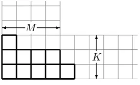
these weights are equivalent to the oscillator numbersnaα andnfa. As discussed above, the grading defines a two-dimensional path. The Young diagram is constructed by drawingνj boxes above thej’th horizontal line, and λaboxes to the right of the a’th vertical line, see figure1.3. From this definition it is clear that a representation ofu(M|K) is characterised by a Young diagram that fits within an L-shaped hook of the form shown in figure 1.4.

Unitarity constraints

Notice that due to the nature of the fermionic duality transformations, the Young diagram is independent of the chosen path. The unitarity constraints (1.12) should hold no matter which grading is chosen. This means that the Young diagrams have to be shaped as a ladder, i.e. the width of the rows have to decrease or remain the same as one goes from below.

Shortening has a very natural interpretation on the level of Young diagrams. A repre-sentation is short if it does not touch the point (M, K) at the corner of the L-hook. See figure1.4 for an example.

Young diagrams as algebra-independent objects

We can just as well describe a Young diagram entirely by the width of its rows, i.e. by a partition λ0 ={λ0

1, ..., λ0H} where H is the height of the first column in the diagram, see figure 1.5. It is clearly not necessary to specify an algebra in order to define the Young

M{

6

? {

K

Figure 1.4: L-hook for u(M|K) with M = 4 and K = 3. The Young diagram specifies a short

yy {{{

y y

λ0_H λ0_H−1 λ0₂ λ0₁

Figure 1.5: Young diagram as a partitionλ0={λ01, ..., λ

0 H}.

diagram. In fact, a diagram characterises an irreducible representation of any u(M|K) algebra for which it fits inside the corresponding L-hook.

Tensor products and trivial extension

The discussion so far has been for abstract representations. If we want to interpret the vector spaces of the representations as tensor products, we need to specify another number: the lengthLof the tensor product or, equivalently, the central chargeC for the individual components in the tensor product. The length and central charge are related to the weights by

L C= M

X

k=1 νk+

K

X

k=1 λk =

H

X

k=1

λ0_k. (1.22)

Let us restrict to the Jordan-Schwinger type representations. As the oscillators fa are fermionic, they can act only once on the vacuum |0i. This means that the allowed representations for the individual components in a tensor product are given by Young diagrams with a single column whose height equals the central charge, see figure 1.6.

C

Figure 1.6: The representation at each site in the tensor product is given by the central chargeC.

1.2. Young diagrams 17

Figure 1.7: Extension of a compact Young diagram. The extension depends on the specification

of a central chargeC, which defines the length through (1.22). Theorange path

cor-responds to the original grading, while theblue path is the extension. The extension

can be arbitrarily big and will have weights{ν1, ..., νM|L, ..., L, λ1, ..., λK,0, ...,0}. In

the depicted example, the u(3|2) partition{4,2,0|4,2}1ˆ12ˆ23 is interpreted as a tensor

product with central chargeC = 2 and thus lengthL= 6. We call the greypart the

trivial extension.

we will refer to this process astrivial extensions. The process is depicted in figure1.7, and it will play a key role in the following.

1.2.2 Non-compact Young diagrams

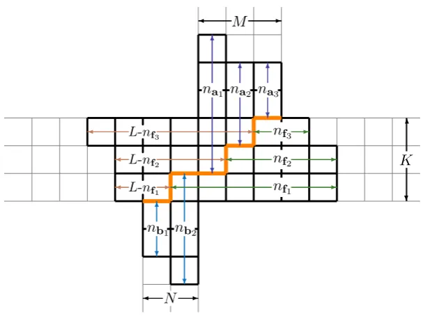
Young diagrams are a standard tool in the analysis of compact representations. In the AdS/CFT integrability context, non-compact representations have previously been classi-fied by diagrams within a T-hook [24,25,26]. In the yet unpublished work on classifications of unitary representations of u(N, M|K) [27], a generalisation of Young diagrams to the non-compact case will be introduced. As a special case of that approach, we now define Young diagrams for a restricted class of irreducible representations. In particular, we want to consider representations that are realised as tensor products of Jordan-Schwinger type representations with integer weights. It is convenient to characterise these representations by the oscillator numbersna,nb and nf rather than their fundamental weights ν and λ. We will discuss the ambiguity in using the fundamental weights after defining non-compact Young diagrams in terms of Jordan-Schwinger oscillators.

Definition in terms of Jordan-Schwinger oscillators

An irreducible representation of u(N, M|K) is characterised by a Young diagram within a grid of the form shown in figure1.8, which we will refer to as aχ-hook. Figure1.8also shows the definition of the Young diagram in terms of the oscillator numbers. Note that it is necessary to specify the central charge C, or, equivalently, the length L. Again, C and Lare related through (1.21).

6

? 6

?

6

? 6

? 6

?

}

nf3

}

nf2

}

nf1

{{

L-nf1

{{

L-nf2

{{

L-nf3

zz

nb1 nzbz2

zz

na1 nzaz2 nzaz3

Nz

M{

6

? {

K

Figure 1.8: Young diagram corresponding to the oscillator numbers na, nf, nb with respect to a

given gradingand a specified central charge C that definesLthrough (1.21). The

ex-ample here corresponds to anu(2,3|3) representation withn1ˆ123ˆ24ˆ35= [2,4|6,4,2|5,3,2]

andC= 0. Consequently,L= 8.

the ˙α’th segment. For the last M horizontal segments, draw naα above the (N +α)’th segment. For the a’th vertical segments, drawnfa boxes to the right andL−nfa boxes to the left.

It is important to note that the above prescription is not valid in all gradings if the representation in question is short. For long representations, the Young diagram touches the start- and end-point of the Dynkin path, which we denote (0,0) and (N+M, K). For short representations, the prescription always yields the correct diagram if one chooses the path

1 2...(N−1)N ˆ1 ˆ2...K−d1 ˆK (N+1) (N+2)...(N+M),

corresponding to ordering the oscillators such that all b oscillators come before all f

oscillators followed by all aoscillators, i.e. u(N,|K|M).

Why the fundamental weights are ambiguous

The above definition of Young diagrams depends on the N+M+K oscillator numbers, but also on the central charge C, or, equivalently, the length L.

1.2. Young diagrams 19

t t

t

t

t

Figure 1.9: Extension of a Young diagram that was originally defined for u(2,2|4) and C = 0

(n12ˆ1ˆ2ˆ3ˆ434 = [2,3|7,6,4,3|2,1]). Thenon-trivial extensionis marked in blue, while the

trivial extensionis marked in grey. The trivial part continues infinitely in the vertical

direction without any horizontal shifts. The central point is marked with a black circle.

The two red points correspond to the algebra u(9), and the shaded boxes show the

corresponding u(9) Young diagram withC = 5. The two greenpoints correspond to

the algebra u(2,4|5) with C = 1. As one of the points is outside the diagram, the

corresponding multiplet is short.

Extension and map to u(N0)

In analogy with the compact case, we would like to think of the non-compact Young diagram as independent of the algebra. Similarly to the compact discussion, we can embed a representation in representations of algebras of higher rank, by extending the set of oscillators and through redefinitions of the Fock vacuum and central charge.

In this procedure, we first extend all rows to have length L. In the upper part of the diagram, we extend the rows towards the left, and in the lower part towards the right. We call this thenon-trivial extension. Above and below this diagram, we place an infinite column of rows that are completely aligned with central vertical line in the diagram. In the upper part, this infinite column is on the left side, while it is on the right side in the lower part. We call this the trivial extension. See figure1.9.

The diagram now corresponds to an irreducible representation of anyu(N, M|K) alge-bra for which it fits inside theχ-hook. An algebra is specified by choosing two points on theZ2 lattice such that the extended Young diagram is between them and that the right point is not lower than the left point. The relative position of these points to one another and to the central vertical line specify the algebra, and the Young diagram then defines an irrep of this algebra. If both points are on the boundary of the extended diagram then this representation is a long multiplet, otherwise it is a short multiplet.

vertical line where the number of boxes that are placed to the left and below the point equals the number of boxesto the right and abovethe point defines the central charge for each component in the tensor product. For u(N, M|K) this point is (N, C+N), since the equality of the number of boxes southwest and northeast of the point,

nb+ N+C

X

a=1

(L−nfa) =na+ K

X

a=N+C+1

nfa , (1.23)

is identical to the central charge constraint (1.21), and we refer to it as the central point or simplycenter of the diagram. Later, we will also refer to it as themomentum-carrying node. Note further that the central vertical line splits the diagram into two halves that are shaped as extended compact diagrams. We call them theleftand right compact diagrams. This gives a way to map u(N, M|K) representations to u(N0) representations, which we will now exploit.

1.3

Characters and counting

Having introduced a way to classify representations, either through the specification of a partition or a Young diagram plus a central charge, we are ready to study the decom-position of tensor product representations into irreps. Representation theory provides a convenient tool in terms of characters.

Character theory for compact representations is described in most textbooks on repre-sentation theory, see e.g. [23]. The generalisation to supersymmetry and non-compactness is less well-studied, and the author is unaware of a treatment combining both features. As proposed in [5], we will use the concept of extended Young diagrams to map u(N, M|K) representations to representations ofu(N0), and thus circumvent the complications arising from supersymmetry and non-compactness. The trade-off is that the rank N0 is un-bounded.

1.3.1 gl(N) characters

The character of an irrep of gl(N) with weights λ = {λ1, ..., λN} is given by the Schur polynomial

χλ =

det1≤i,j≤Nx λj+N−j i det1≤i,j≤NxN_i −j

≡ Wλ

∆V , (1.24)

where the denominator ∆V =Q

i<j(xi−xj) is the Vandermonde determinant.

We are particularly interested in tensor products of such irreps. A tensor product representation is reducible, and it can be written as a direct sum of irreps,

λ⊗˜λ=M i

1.3. Characters and counting 21

The character of the tensor product representation is simply the product of the characters of its factors, i.e.χ_λ⊗L =χL_λ. At the same time, the character of a reducible representation is a sum of characters of irreps:

χreducible=X λ

cλχλ, (1.26)

and the integer multiplicities cλ are uniquely determined. In the case of the L’th tensor product of an irrep λ, we get

χL_λ =X λ0

cλ0χ_λ0. (1.27)

Actually, the polynomial Wλ = ∆V ·χλ is more convenient to work with. For a given representationλ,Wλ will contain a term of the kind

xλ1+N−1

1 x

λ2+N−2 2 · · ·x

λN−1+1 N−1 x

λN

N , (1.28)

which we will call the dominant term. The advantage of W compared to χ is that the dominant terms are unique toWλ, i.e. they do not appear in Wλ0 ifλ6=λ0. We can then effectively decompose into irreps by reading off the coefficient of the dominant terms in the expression

∆V ·χreducible=

X

λ

cλWλ. (1.29)

1.3.2 Polya theory

The tensor product character (1.27) can be seen as a sum of all the states in the spectrum with length L. In the next section, we will want to interpret single-trace operators in N = 4 SYM as tensor product states. The trace is cyclic, which means that tensor product states that are related by cyclic permutations, i.e. by the cyclic group ZL, are considered to be equivalent. This effectively reduces the size of the vector space of states. The above analysis does not take this property into account.

The Polya theorem [28]1 provides a way to account for equivalence relations between

tensor product states, in our case cyclic permutations. According to the Polya theorem, the tensor product character (1.27) should be replaced by the reduced sum of states ZL given by

ZL=

X

d|L φ(d)

L χ1(x d

1, ..., xdN) L

d . (1.30)

Here d|L denotes all divisors of L, while φ(d) is the Euler totient function given by the number of integers between 1 and dthat are mutually prime withd. χ1 is the character of the representation that each component of the tensor product is in.

1

The practical usage of characters is demonstrated in appendix A.2, both in simple examples and to understand the multiplet content in N = 4 SYM, towards which we now turn our focus.

1.4

The

N

= 4

SYM spectrum

Our goal is to classify the symmetry multiplets formed by single-trace operators inN = 4 SYM. Such a classification was first done in [30] and further investigations made in [31].

The superconformal algebra is isomorphic topsu(2,2|4). The generators of the symme-try can be realised as differential operators on the fundamental fields that constitute local operators, and as such, they act via the chain rule. This fits well with the action of ab-stract symmetry generators on a tensor product, and thus we can interpret the composite operators as tensor products.

At zero coupling, i.e.g→0, the symmetry is in fact enhanced topu(2,2|4)⊕u(1), where the extra u(1) corresponds to the fixed length L. This section reviews how multiplets of single-trace operators are affected by this transition in symmetry induced by turning on the coupling.

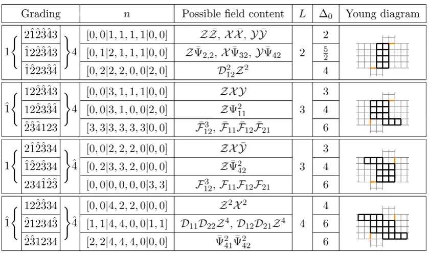
1.4.1 Field interpretation of states

The states satisfying the central charge constraintC= 0 and their interpretation in terms of fields inN = 4 SYM are summarised in table1.1. The fields correspond to an infinite-dimensional representation reflecting the possibility of acting with an arbitrary number of covariant derivatives on each field. The corresponding pu(2,2|4) Young diagram is depicted in figure 1.10. The fields are assigned a classical conformal dimension, ∆0, given

Field interpretation Content ∆0 Components

scalar Φab fa†f_b†|0i 1 6

fermion Ψaα f

†

aa†α|0i 3₂ 8 ¯

Ψaα˙ abcdf

†

bf

†

cf_d†b†_α˙|0i 3₂ 8 field strength Fαβ a

†

αa†_β|0i 2 3 ¯

F_α˙β˙ f₁†f₂†f₃†f₄†b†_α˙b†_˙

β|0i 2 3 covariant derivative Dαα˙ a†αb†_α˙ 1 4

Table 1.1: States satisfying the central charge constraint. Note that Φab = −Φba, i.e. there are

six independent scalars. We denote them by Z ≡f1†f

†

2|0i, X ≡ f

†

1f

†

3|0i, Y ≡ f

†

1f

†

4|0i, ¯

Y ≡f₂†f₃†|0i, ¯X ≡f₂†f₄†|0i, ¯Z ≡f₃†f₄†|0i. Note also thatFαβ =Fβα and ¯Fα˙β˙ = ¯Fβ˙α˙. A

state can contain one of the fundamental fields and an unlimited number of covariant

1.4. The N = 4 SYM spectrum 23

t

Figure 1.10: (left) Theχ-hook and the Young diagram corresponding to the single-field

representa-tion inN = 4 SYM. The central point is marked. (right) The extended Young diagram

corresponding to the single-field representation.

by

∆0= nf

2 +na. (1.31)

Composite operators made of Lfields are interpreted as tensor products of Lvectors from the above representation. As an example, consider theL= 3 state

Tr[Z D12Ψ11 F12] =f₁†f₂†|0i ⊗(a†₁)2b†₂f₁†|0i ⊗a†₁a†₂|0i. (1.32) For simplicity, we will often leave out the Tr[...] symbol. Cyclicity of the trace means that two states are equivalent if they are related by cyclic permutations, e.g. ZX = X Z. As fermions anti-commute, this also means that some states involving fermions vanish, e.g. ΨaαΨaα=−ΨaαΨaα= 0. The central charge constraint for a tensor product state is

na−nb+nf = 2L , (1.33)

and this definesL through the oscillator numbers.

pu(2,2|4) Young diagrams

The Young diagrams of the irreps of pu(2,2|4) are drawn within the χ-hook shown in figure1.10. We will refer to the point (2,2) as thecentral point. It splits the diagram into four quadrants. The central charge constraint C = 0 manifests itself as the demand that the number of boxes in the upper-right and lower-left quadrants must be equal, see figure 1.11. Furthermore, the left and right half of the diagram should be of ladder shape [27]. The unitarity constraints (1.12) only demands this for the four middle rows, but it turns out that diagrams which are not of ladder-shape correspond to operators that are set to zero by the equations of motions. An example is the diagram on the right in figure 1.11 (nyp _{= [1,1|1,1,1,1|1,1] in the notation introduced below), which corresponds to a HWS} of the formabcdΦabΦcd. The equations of motion are realised in the oscillator language as=αβ_α˙β˙Dαα˙D_ββ˙ = det

1≤α,α˙≤2a

†

t t

Figure 1.11: (left) An example of apu(2,2|4) diagram having the same number of boxes in the

lower-leftandupper-rightquadrant. (right) A Young diagram that is not ladder-shaped and

allowed by thepu(2,2|4) unitarity constraints (1.12), but corresponds to an operator

that is zero due to the equations of motion.

1.4.2 Quantum numbers and finite g

At zero coupling, the multiplets of operators are representations of pu(2,2|4)⊕u(1). As such, we need eight numbers to classify the representations. As mentioned, we will prefer to use the oscillator numbers to classify representations. We will do this in the notation

ngrading= [nb1, nb2|nf1, nf2, nf3, nf4|na1, na2], (1.34)

where the oscillator numbers are those of the HWS with respect to the specified grading. Our preferred choice of grading will be 12ˆ1ˆ2ˆ3ˆ434, also known as thecompact beautygrading [32], for which we will use the symbolyp as a short-hand notation referring to its Dynkin path. This choice is convenient since it minimises the classical conformal dimension (1.31).

Turning on g

The above use of Jordan-Schwinger oscillators is only an adequate description of N = 4 SYM atg= 0. The Jordan-Schwinger-type representations have integer weights, and this is no longer true wheng6= 0. Understanding the nature of the representations formed by single-trace operators at finite coupling is still an unsolved, and very interesting, problem. The global symmetry of N = 4 SYM has the two bosonic subalgebras su(4) and

su(2,2). The su(4) part corresponds to the R-symmetry and is related to the S5 part of the dual geometry. The corresponding weightsλado not run with the coupling and remain integers at any coupling. The su(2,2) part, related to the conformal symmetry and the AdS5 part of the dual geometry, is not as simple. The conformal symmetry includes the dilatation operator, and as it is renormalised, the weights of this part of the symmetry, νi, run with the coupling since they contain the anomalous dimension. The behaviour is

νi = νi|g=0+ γ

1.4. The N = 4 SYM spectrum 25

nyp L Field content example λa νj

[1,1|2,2,2,2|1,1] 4 Ψ11Ψ12Ψ¯11Ψ¯12 {2,2,2,2} {−5,−5,1,1} [0,0|2,2,2,2|1,1] 5 Ψ11Ψ12Z¯X¯Y¯ {2,2,2,2} {−5,−5,1,1} [1,1|3,3,3,3|0,0] 5 Ψ¯11Ψ¯12ZX Y {3,3,3,3} {−6,−6,0,0}

Table 1.2: Three types of operators with differing oscillator content and length that have the same

psu(2,2|4) quantum numbers: λa−λa+1={0,0,0}andνj−νj+1={0,−6,0}.

At finite coupling, the multiplets organise themselves in representations of psu(2,2|4). Such representations are characterised by just six numbers. A choice is the differences of the fundamental weights λa−λa+1 and νj −νj+1. Note that the weights {λ, ν} and {λ+ Λ, ν−Λ}define isomorphic irreps of psu(2,2|4).

The relation between oscillator numbers and other conventionally used parametrisa-tions of thepsu(2,2|4) quantum numbers are given in appendixA.1. Despite the obscured interpretation at finite coupling, we will prefer to label multiplets by the HWS oscilla-tor content (1.34) that they flow towards as g → 0, since this classification contains the complete information, and since our main objective is perturbative calculations.

Length mixing

At finite coupling, the notion of a length breaks down. In general, the eigenstates of the dilatation operator is a mix of any operator with the same psu(2,2|4) quantum numbers [33]. On the level of level of oscillators, the length can be changed by two transformations that leave the differences λa−λa+1 and νj−νj+1 invariant:

{L, n_bα˙} ↔ {L−1, nbα˙+1}, (1.36a) {L, n_fa, naα} ↔ {L−1, nfa−1, naα+1} (1.36b)

Note that (1.36a) leavesλandνinvariant, while (1.36b) takesλa↔λa−1 andνi ↔νi+1. An example of operators related by these transformations and consequently able to mix at higher loops is given in table1.2.

1.4.3 Shortening and joining

As discussed, shortening happens whenever λa+νj = 0. At g = 0 this happens for all multiplets that correspond to diagrams not touching the edges of theχ-hook. This means that some fermionic duality transformations do not alter the HWS.

70 possible Dynkin paths on the 4|4 lattice. The only explanation of this phenomenon is that the shortpu(2,2|4)⊕u(1) multiplets must combine into largerpsu(2,2|4) multiplets.

Protected operators: the BMN vacuum

There is one type of multiplet that is not subject to joining: the multiplets containing the states TrZL_{. The oscillator numbers are}

nyp = [0,0|L, L,0,0|0,0]. (1.37)

Due to the fact that they are annihilated by half the supercharges, these operators are protected from quantum corrections and have vanishing anomalous dimension, see e.g. [11].

Shortening conditions

The non-trivial unitarity bounds are

λ1+ν1 ≤ 0, (1.38a)

λ4+ν4 ≥ 0. (1.38b)

These bounds must be satisfied by any member of a multiplet. For this, we need to require that (1.38a) holds for gradings of the type{1ˆ1}..., and that (1.38b) holds for gradings of the type...{4ˆ4}. Here the notation{ab}means that aand bcan be in either order.

Shortening happens when one or both bounds are saturated, i.e. when

λ1+ν1 = nf1−L−nb1 = 0, (1.39a)

λ4+ν4 = nf4+na2 = 0, (1.39b)

which we refer to as shortening conditions. On the level of oscillators, the condition (1.39a) can only happen if nf1 =L and nb1 = 0. Similarly, (1.39b) implies nf4 = na2 = 0. Shortenings rule out the possibility of the length-changing replacements (1.36). In particular, (1.39a) rules out (1.36a) and (1.39b) rules out (1.36b).

Joining

Let us take a short multiplet and reconsider what happens during fermionic duality trans-formations that leave the HWS unchanged.

Consider a multiplet subject to the shortening (1.39a). The oscillator content in a grading of the type 1ˆ1... must be of the form

[0, nb2|L,•,•,•|•,•] L

1.4. The N = 4 SYM spectrum 27

1...4 ˆ1...4 1...ˆ4 ˆ1...ˆ4

Figure 1.12: Example of four different Young diagrams for short multiplets that join into one at

finite coupling. The changes with respect to the diagram on the left are highlighted.

where the length and grading is specified in super- and subscript. If the multiplet was long, the effect of the duality transformation to the ˆ11... grading would be {λ1, ν1} → {λ₁ + 1, ν1 −1}, which seems to give the inadmissible oscillator content [1, nb2|L + 1,•,•,•|•,0]L_ˆ11.... However, this can be cured by the length-changing replacement (1.36a). The resulting oscillator numbers are

[0, nb2 −1|L+ 1,•,•,•|•,•] L+1 ˆ

11.... (1.40b)

This is how joining works: shortpu(2,2|4)⊕u(1) multiplets of different lengths join into one

psu(2,2|4) multiplet. A similar treatment reveals that multiplets subject to the shortening (1.39b) combine as

[•,•|•,•,•,0|na1,0] L

...ˆ44, (1.41a)

[•,•| •+1,•+ 1,•+ 1,0|na1 −1,0] L+1

...4ˆ4 . (1.41b) If both shortenings (1.39) happen, the four multiplets

[0,•|L,•,•,0|•,0]L_1...4, [0,• −1|L+ 1,•,•,0|•,0]L_ˆ+1

1...4, [0,•|L+ 1,•+ 1,•+ 1,0| • −1,0]L+1

1...ˆ4, [0,• −1|L+ 2,•+ 1,•+ 1,0| • −1,0]L_ˆ+2

1...ˆ4, (1.42) join into one.

In table1.3we give examples of the different members of the short Konishi multiplet. We also display the joining on the level of Young diagrams in figure 1.12. Note that two identical Young diagrams can appear in different types of long multiplets as they can describe the HWS in different gradings.

Stronger shortenings

Grading n Possible field content L ∆0 Young diagram

1

( 2ˆ1ˆ2ˆ3ˆ43 )

4

[0,0|1,1,1,1|0,0] ZZ¯,XX¯,YY¯

2 2 ˆ

12ˆ2ˆ3ˆ43 [0,1|2,1,1,1|0,0] ZΨ¯2,2,XΨ¯32,YΨ¯42 5₂ ˆ

1ˆ223ˆ3ˆ4 [0,2|2,2,0,0|2,0] D2

12Z2 4

ˆ 1

( 12ˆ2ˆ3ˆ43 )

4

[0,0|3,1,1,1|0,0] ZX Y

3 3 12ˆ23ˆ3ˆ4 [0,0|3,1,0,0|2,0] ZΨ2₁₁ 4 ˆ

2ˆ3ˆ4123 [3,3|3,3,3,3|0,0] F¯3

12, ¯F11F¯12F¯21 6

1

( 2ˆ1ˆ2ˆ334 )

ˆ 4

[0,0|2,2,2,0|0,0] ZXY¯

3 3 ˆ

1ˆ22ˆ334 [0,2|3,3,2,0|0,0] ZΨ¯2₄₂ 4 234ˆ1ˆ2ˆ3 [0,0|0,0,0,0|3,3] F3

12,F11F12F21 6

ˆ 1

( 12ˆ2ˆ334 )

ˆ 4

[0,0|4,2,2,0|0,0] Z2_X2 ₄ ˆ

21234ˆ3 [1,1|4,4,0,0|1,1] D11D22Z4,D12D21Z4 4 6 ˆ

2ˆ31234 [2,2|4,4,4,0|0,0] Ψ¯2₄₁Ψ¯2₄₂ 6

Table 1.3: Selected components of the Konishi multiplet, which splits into four short multiplets at

g= 0.

be a HWS in the grading ˆ112... at finite coupling. Similarly, the case nf1 =nf2 =L and nb1 = 0 implies the 1ˆ1ˆ2... grading. If (1.39b) is supplemented by na2 = 0 it implies the grading...34ˆ4, and if supplemented bynf3 = 0 it implies ...ˆ3ˆ44 at finite coupling.

There is one scenario that the joining mechanism cannot handle: if both nb2 = 0 in the {1ˆ12}... gradings and nf2 = L in the {1ˆ1ˆ2}... gradings. The only multiplets in the N = 4 spectrum with this property are the protected BMN vacua discussed above which remain short at finite coupling.

1.4.4 Sectors

Shortening is crucial in understanding the appearance of closed sectors of operators. By

a closed sector, we refer to operators with restricted field content that do not mix with

operators with different field content, i.e. the eigenstates of the dilatation operator will be a linear combination of single-trace operators of only this kind at any coupling. This is the case when thepsu(2,2|4) quantum numbers, i.e. the six numbersλa−λa+1 andνj−νj+1, can only be used to construct certain fields.

In a closed sector, some oscillators are passive in the sense that they are either saturated (e.g.nf1 =L) or not excited at all (e.g.nf4 = 0), while some oscillators are excited and form a set of non-trivial raising operators. Furthermore, the length-changing transformations (1.36a) and (1.36b) do not excite the passive oscillators.

1.4. The N = 4 SYM spectrum 29

Rank 1 2 3 4 5 6

su(2)

su(1|1)

su(1,|1)

su(1,1)

su(1|2)

su(1,|2)

su(1,1|1)b

su(1,1|1)a

psu(1,1|2)

su(2|3)

su(2,|3)

su(1,2|2)

su(2,1|2)

su(1,2|3)

su(2,1|3)

psu(2,2|4)

Figure 1.13: Closed sectors. lcompactlnon-compact.

the su(1,1) = sl(2) sector combines the fourth and sixth type: [0,•|L, L,0,0|•,0], while thesu(2,1|3) sector is of the second type: [•,•|•,•,•,0|•,0]. All closed sectors are listed in table1.5. The rank of the sector is one lower than the number of active oscillators. The sectors of low rank are subsectors of those of higher rank, and the relationship between sectors is summarised in figure1.13.

Note that in sectors where only one of the shortening conditions (1.39) is satisfied, one of the length changing transformations (1.36) is allowed and results in an operator with the same psu(2,2|4) quantum numbers, but with a different length. As discussed, this means that at higher loops the eigenstates of the dilatation operator can mix operators of different length.

Figure 1.14shows the Young diagrams for multiplets containing operators in thesl(2) and su(2) sectors. Note that the multiplets nyp _{= [0,0|L−1, L− 1,1,1|0,0] contain} operators from all sectors.

[nb|nf|na] Grading [0,•|L,•,•,•|•,•] {1ˆ1}... [•,•|•,•,•,0|•,0] ...{4ˆ4} [0,0|L,•,•,•|•,•] ˆ112... [0,•|L, L,•,•|•,•] 1ˆ1ˆ2... [•,•|•,•,•,0|0,0] ...34ˆ4 [•,•|•,•,0,0|•,0] ...ˆ3ˆ44

Table 1.4: Types of shortening and resulting grading for the state that remains a HWS at finite

coupling. Brackets{}denote interchangeable gradings.

1.4.5 Counting multiplets

In the AdS5/CFT4 context the counting of multiplets was done in [29,34] by engineering

sl(2) su(2)

L−1

L−1 L−1

L−1

S

−

2

S

−

2

L−3 L−M−1

M−1

M−1 L−M−1

L−3

Figure 1.14: Young diagrams (of yp HWS) for multiplets containing sl(2), DS

12ZL, and su(2),

ZL−MXM

, operators.

diagrams can in fact be seen as representations ofu(4 +nyp_b2+nyp_a1) with central chargeC= 2+nyp_b

2. We can exploit this to apply the tools of section1.3to count the multiplets inN = 4 SYM. An important point is that it is possible to make a cut-off in the classical dimension given by (1.31). To account for all multiplets up to a maximal classical dimension ∆yp_0,max of the HWS in the ypgrading, it is sufficient to consideru(2∆yp_0,max) representations where the tensor product components are in representations with central charge C= ∆yp_0,max, cf. (1.30). Details of such calculations are given in appendixA.2. Table1.6gives an overview of the multiplets with ∆yp

0 ≤5.5. See appendixA.3for a list of all multiplets with ∆yp0 ≤8.

Subconclusion

In this chapter, we have seen how to construct and classify Jordan-Schwinger type rep-resentations of u(N, M|K) in terms of oscillators and Young diagrams. By introducing the idea of extended Young diagrams, we have seen how to use standard Schur polynomi-als to decompose tensor products of non-compact representations into irreps, polynomi-also taking cyclic equivalence into account. We then applied this framework to the global symmetry of N = 4 SYM in the limitg → 0. We saw how its representations quite magically glue together at finite coupling to form longpsu(2,2|4) multiplets.

1.4. The N = 4 SYM spectrum 31

Rank Sector Field content [nb|nf|na] Grading(s)

1

su(1,1) DS

12ZL [0, S|L,L,0,0|S ,0] 1ˆ1ˆ223ˆ3ˆ44 su(1,|1) ZL−N_Ψ¯N

42 [0, N|L,L, N ,0|0,0] 1ˆ1ˆ2[2ˆ3]34ˆ4 su(1|1) ZL−N_ΨN

11 [0,0|L, L−N ,0,0|N ,0] ˆ112[3ˆ2]ˆ3ˆ44 su(2) ZL−M_XM _{[0, 0|L, L−M , M ,0|0,0] ˆ112ˆ2ˆ334ˆ4}

2

su(1,1|1)a D12SZL−NΨN11 [0, S|L, L−N ,0,0|S+N ,0] {1ˆ1}[23ˆ2]ˆ3ˆ44 su(1,1|1)b DS

12Z L−N_Ψ¯N

42 [0, S+N|L,L, N ,0|S,0] 1ˆ1ˆ2[23ˆ3]{4ˆ4} su(1,|2) ZL−M−N_XM_Ψ¯N

42 [0, N|L, L−M , M+N ,0|0,0] {1ˆ1}[2ˆ2ˆ3]34ˆ4 su(1|2) ZL−M−N_XM_ΨN

11 [0,0|L, L−M−N , M ,0|N ,0 ] ˆ112[3ˆ2ˆ3]{4ˆ4} 3 psu(1,1|2) D

S

12ZL−M−N1−N2+S

XM+S_ΨN1−S 11 Ψ¯

N2−S 42

[0, N2|L, L−M−N1, M+N2,0|N1, 0]

{1ˆ1}[23ˆ2ˆ3]{4ˆ4}

4

su(2,1|2) D S1 11D

S2 12Z

L−N1−N2+n

ΨN1−n 11 Ψ

N2−n 21 F11n

[S1, S2|L−N2, L−N1, 0,0|N1+N2+S1+S2,0]

[123ˆ1ˆ2]ˆ3ˆ44

su(2,|3) Z

L−M1−M2−N1−N2

XM1_Y¯M2_Ψ¯N1 42Ψ¯

N2 41

[N2, N1|L−M2, L−M1, M1+M2+N1+N2,0|0,0]

[12ˆ1ˆ2ˆ3]34ˆ4

su(1,2|2) D S1 12D

S2

22ZL−N1−N2+n ¯

ΨN1−n 42 Ψ¯

N2−n 32 F¯22n

[0, S1+S2+N1+N2|L,L, N1, N2|S1, S2]

1ˆ1ˆ2[234ˆ3ˆ4]

su(2|3) Z

L−M1−M2−N1−N2

XM1_YM2_ΨN1 11Ψ

N2 12

[0,0|L, L−M1−M2−N1−N2, M1, M2|N1, N2]

ˆ

112[34ˆ2ˆ3ˆ4]

5

su(1,2|3) D •

12D•22X•Y•Z• Ψ₁₁• Ψ•₁₂Ψ¯•₄₂Ψ¯•₃₂Ψ¯•₂₂F¯•

22

[0,•|L,•,•,•|•,•] [123ˆ1ˆ2ˆ3]{4ˆ4}

su(2,1|3) D •

11D•12X•Y¯•Z• ¯

Ψ•₄₂Ψ¯•₄₁Ψ₁₁• Ψ•₂₁Ψ•₃₁F11•

[•,•|•,•,•,0|•,0] {1ˆ1}[234ˆ2ˆ3ˆ4]

Table 1.5: Closed sectors. Passive oscillators are marked in grey. A bracket [ ] denotes duality

transformations that shuffle active oscillators and change the HWS within the sector

while preserving the length. A bracket{}denotes a duality transformation that shuffles

passive oscillators and changes the HWS within the sector while changingL. Note that

the field content in thepsu(1,1|2),su(2,1|2),su(1,2|2),su(2,1|3) andsu(1,2|3) sectors is

not completely fixed by the oscillator numbers, but they can still be considered sectors

∆yp

0 L [nb|nf|na]yp S1 S2 Sector Multiplicity 2 2-4 [0,0|1,1,1,1|0,0] _{4 4} all 1 3 3-5 [0,0|2,2,1,1|0,0] _{4 4} all 1

4

4-6 [0,0|3,3,1,1|0,0] _{4 4} all 2 3-5 [0,1|2,2,1,1|1,0] 4 4 sl(2) 2 2-4 [0,2|1,1,1,1|2,0] _{4 4} sl(2) 1 4-6 [0,0|3,2,2,1|0,0] _{4 4} su(2) 1 3-4 [0,0|1,1,1,1|2,0] 8 4 su(2,1|2) 1 [0,2|2,2,2,2|0,0] _{4 8} su(1,2|2) 1 4 [0,0|2,2,2,2|0,0] _{8 8} psu(2,2|4) 2

5

5-7 [0,0|4,4,1,1|0,0] _{4 4} all 2 4-6 [0,1|3,3,1,1|1,0] _{4 4} sl(2) 2 3-5 [0,2|2,2,1,1|2,0] _{4 4} sl(2) 1 5-7 [0,0|4,3,2,1|0,0] 4 4 su(2) 2 4-6 [0,0|3,1,1,1|2,0] 4 4 su(1|1) 1

[0,2|3,3,3,1|0,0] su(1,|1) 1 4-6 [0,1|3,2,2,1|1,0] 4 4 psu(1,1|2) 4 5-6 [0,0|3,3,3,1|0,0] 8 4 su(2,|3) 2 [0,0|4,2,2,2|0,0] _{4 8} su(2|3) 2 4-5 [0,0|2,2,1,1|2,0] 8 4 su(2,1|2) 2 [0,2|3,3,2,2|0,0] _{4 8} su(1,2|2) 2 5 [0,0|3,3,2,2|0,0] _{8 8} psu(2,2|4) 4 4 [0,1|2,2,2,2|1,0] _{8 8} psu(2,2|4) 2

11 2

5-7 [0,0|4,3,1,1|1,0] 4 4 su(1|1) 2

[0,1|4,4,2,1|0,0] su(1,|1) 2 4-6 [0,1|3,2,1,1|2,0] _{4 4} su(1,1|1)a 2 [0,2|3,3,2,1|1,0] su(1,1|1)b 2 3-5 [0,2|2,1,1,1|3,0] _{4 4} su(1,1|1)a 2 [0,3|2,2,2,1|2,0] su(1,1|1)b 2 5-6 [0,0|3,3,2,1|1,0] 8 4 su(2,1|3) 4 [0,1|4,3,2,2|0,0] _{4 8} su(1,2|3) 4 4-5 [0,1|2,2,2,1|2,0] 8 4 su(2,1|3) 4 [0,2|3,2,2,2|1,0] _{4 8} su(1,2|3) 4 5 [0,0|3,2,2,2|1,0] _{8 8} psu(2,2|4) 4 [0,1|3,3,3,2|0,0] 4

Table 1.6: All unprotected multiplets for which ∆yp0 ≤11₂. The columns S1 and S2 denote whether

Chapter 2

Spin chains and integrability

We call a modelquantum integrable if it falls within the framework of Bethe ansatz tech-niques, where the Yang-Baxter equation is the basic prerequisite. This chapter gives a practical and informal review of these frameworks, and the discussion will progress through explicit examples. To avoid getting lost in tedious notation, we will introduce the techniques in a model with su(2) symmetry, the Heisenberg spin chain, and comment on the generalisation to higher rank symmetry at the end of the chapter. The main goal is to introduce the concept of a Q-system, which plays a central role throughout the thesis.

2.1

The Heisenberg spin chain and coordinate Bethe ansatz

The Heisenberg spin chain is not only a convenient toy model on which the tools of integrability can be demonstrated, it also describes the one-loop spectrum of the su(2) sector inN = 4 SYM.

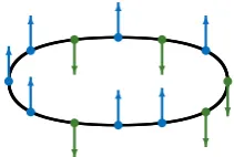
2.1.1 The closed Heisenberg spin chain

Consider a one-dimensional model ofL spins, which are all in the same representation of some Lie algebra, with periodic boundary conditions, see figure2.1. In the Heisenberg spin chain, these spins belong to the two-dimensional fundamental representation ofsu(2), and we denote the statesspin up↑andspin down↓. The model is specified by the Hamiltonian

H = L

X

k=1

(I−Pk,k+1), (2.1)

wherePi,j is the permutation operator that interchanges the spins at positioniand j. As the chain is closed, we identify thek’th and the (L+k)’th site, i.e.PL,L+1=PL,1. Notice that the Hamiltonian only contains interactions between neighbouring spins.

Through the per