ABSTRACT
O’BRIEN, MICHAEL PATRICK. A Multifaceted Approach to Improving the Practicality of Structural Graph Algorithms. (Under the direction of Blair D. Sullivan.)
Graph algorithms have become an integral part of modern data analytics, but existing ap-proaches have struggled to scale to increasing network sizes. The theoretical computer science community has a rich history of research that circumvents these scalability issues through algorithms that exploit the structural sparsity of graphs. Because many real-world networks from diverse domains are known to share properties like sparsity, clustering, and heavy-tailed degree distributions, structure-based algorithms appear on the surface to be an attractive alternative. However, they come with their own set of problems, such as non-constructive proofs, massive constants hidden in big-O notation, and attention paid to exploiting structures that are unlikely to occur in real data. Consequently, there is a large gap between the most theoretically efficient algorithms and the most practical ones.
A Multifaceted Approach to Improving the Practicality of Structural Graph Algorithms
by
Michael Patrick O’Brien
A dissertation submitted to the Graduate Faculty of North Carolina State University
in partial fulfillment of the requirements for the Degree of
Doctor of Philosophy
Computer Science
Raleigh, North Carolina 2018
APPROVED BY:
Carla D. Savage Matthias F. Stallmann
Steffen Heber Blair D. Sullivan
DEDICATION
BIOGRAPHY
ACKNOWLEDGEMENTS
TABLE OF CONTENTS
LIST OF TABLES . . . viii
LIST OF FIGURES . . . ix
Chapter 1 Introduction . . . 1
1.1 Motivation . . . 1
1.2 Overarching Challenges . . . 2
1.3 Research Questions and Outline . . . 3
Chapter 2 Background. . . 4
2.1 Graph Theory . . . 4
2.2 Sparse Graph Hierarchy . . . 5
2.2.1 Treedepth . . . 6
2.2.2 Excluded Minors . . . 8
2.2.3 Bounded Expansion . . . 9
2.2.4 Nowhere/Somewhere Density . . . 11
2.2.5 Degeneracy and Core Decompositions . . . 12
2.3 Random Graph Models . . . 13
2.3.1 Asymptotic Properties . . . 13
2.3.2 RGMs with Bounded Expansion . . . 13
2.4 Parameterized Complexity . . . 15
2.4.1 Relationship to Graph Structure . . . 16
2.4.2 Parameterized Lower Bounds . . . 16
Chapter 3 Locally Estimating Core Numbers . . . 18
3.1 Introduction . . . 19
3.2 Related Work . . . 21
3.3 Local Estimation . . . 21
3.3.1 Neighborhood-based Estimation . . . 21
3.3.2 Structures Leading to Error . . . 25
3.3.3 Expected Behavior on Random Graphs . . . 26
3.4 Experimental Results . . . 27
3.4.1 Methods . . . 28
3.4.2 Results . . . 28
3.5 Network Treatment . . . 33
3.5.1 Problem Statement . . . 33
3.5.2 Estimatingk-core Exposure Probabilities . . . 35
3.6 Conclusion . . . 37
Chapter 4 CONCUSS . . . 40
4.1 Introduction . . . 41
4.2 Algorithmic Landscape for Classes of Bounded Expansion . . . 41
4.3.1 Motif Counting . . . 42
4.3.2 Graphlet Degree Distribution . . . 43
4.3.3 Existing Algorithms . . . 43
4.4 CONCUSS . . . 45
4.4.1 Color . . . 47
4.4.2 Decompose . . . 48
4.4.3 Compute . . . 48
4.4.4 Combine . . . 49
4.4.5 Extensions to other problems . . . 49
4.5 Experimental Design . . . 49
4.5.1 Data . . . 50
4.5.2 Hardware . . . 50
4.6 Competitive Evaluation . . . 50
4.6.1 Configuration Testing . . . 51
4.6.2 Comparison withNXVF2 . . . 53
4.7 Bottleneck Identification . . . 55
4.7.1 Color Class Distribution . . . 55
4.7.2 Color Set Treedepth . . . 58
4.8 Conclusion . . . 59
Chapter 5 Linear Colorings . . . 60
5.1 Introduction . . . 61
5.2 p-Linear and Linear Colorings . . . 61
5.3 Lower Bounds . . . 63
5.4 Upper Bounds on Trees . . . 66
5.5 Upper Bounds on Interval Graphs . . . 68
5.6 Hardness of Recognizing Linear Colorings . . . 71
5.7 Conclusion . . . 74
Chapter 6 Identifying Dense Substructures . . . 75
6.1 Introduction . . . 76
6.2 Background . . . 77
6.3 Algorithmic Considerations . . . 78
6.4 NP-Hardness . . . 80
6.5 ETH Lower Bounds . . . 86
6.6 Conclusion . . . 89
Chapter 7 Local Search . . . 91
7.1 Introduction . . . 91
7.2 Background . . . 94
7.2.1 Notation . . . 94
7.2.2 Problem Definitions . . . 94
7.3 Algorithmic Strategy . . . 94
7.4 Vertex Cover . . . 95
7.4.2 Correctness . . . 96
7.4.3 Weighted Variant . . . 98
7.5 Maximal Matching . . . 99
7.5.1 Algorithm Description . . . 100
7.5.2 Correctness . . . 101
7.5.3 Weighted Variant . . . 104
7.6 Conclusion . . . 105
Chapter 8 Interdisciplinary Applications . . . 106
8.1 Introduction . . . 107
8.2 Background . . . 108
8.2.1 De Bruijn Graphs . . . 108
8.2.2 Data . . . 108
8.2.3 Evaluation Metrics . . . 109
8.3 Neighborhood Indexing . . . 109
8.3.1 Algorithmic Description . . . 109
8.3.2 Biological Impact . . . 110
8.4 The CAtlas . . . 112
8.4.1 Description . . . 112
8.4.2 CAtlas Construction . . . 112
8.4.3 Biological Impact . . . 114
8.5 CAtlas Search . . . 114
8.5.1 Algorithmic Description . . . 114
8.5.2 Query Preprocessing . . . 115
8.5.3 Biological Impact . . . 115
8.6 Beyond Metagenomics . . . 115
8.7 Conclusion . . . 116
Chapter 9 Conclusion & Future Work . . . 118
BIBLIOGRAPHY . . . .121
APPENDIX . . . 129
LIST OF TABLES
Table 3.1 Summary statistics for real-world graphs used in evaluating local core estimators. . . 28 Table 3.2 Proportion of vertices inNδ. Values less than .01 rounded to 0. . . 32
Table 4.1 Average run time and dynamic programming operations used for each color splitting heuristic. The statistics for med and min are reported as percent increases over max. . . 57 Table 4.2 Average execution time per operation and average depth of vertices in
LIST OF FIGURES
Figure 2.1 An artistic rendering of the sparse graph hierarchy by Felix Reidl. . . . 6 Figure 3.1 The core numberk(v)is they-value at intersection of two functions. . 23 Figure 3.2 T2,4is in blue. T2,40 isT2,4plus w1,w2 (red), and the dashed edges. . . . 25 Figure 3.3 Core number distribution for the real world networks in Table 3.1. . . . 29 Figure 3.4 Proportion of vertices with optimal core number estimate ratios for the
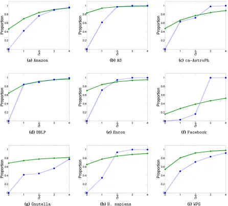
propagating (solid green) and induced (dashed blue) estimators as a function ofδ. . . 30
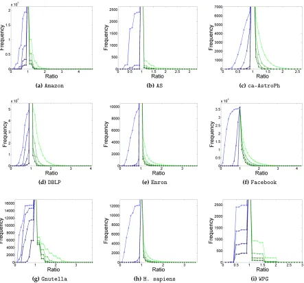
Figure 3.5 Number of vertices with core number estimate ratios less optimal that a given threshold fromδ =1 (lightest line) toδ =4 (darkest line). ˆkδ is
shown in green while ˘kδis shown in blue. Because the number of vertices
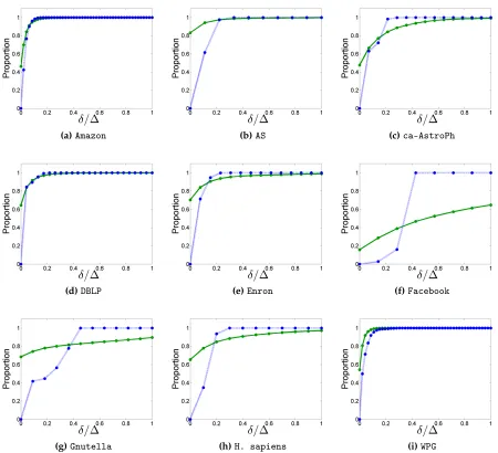
with optimal ratios is frequently large (see Figure 3.4), the vertices with optimal ratios may not appear within the limits of the plot in order better capture the distribution of those vertices with suboptimal ratios. . . 31 Figure 3.6 Average proportion of vertices in Nδ as a function ofδ/∆. . . 32
Figure 3.7 Proportion of vertices with optimal core number estimate ratios for the propagating estimator (solid green) and the induced estimator (dashed blue) as a function of δ. The x-axis has been normalized by the diameter. 34
Figure 3.8 T3,30 with 13 of 16 vertices treated. k(v) = k(u1) = k(u2) = k(u3) = 3. Althoughv,u1,u2, andu3 have all of their neighbors treated, they only have core number 1 with respect to the treated subgraph. . . 36 Figure 3.9 P[Xκ(d)]−P[Xˆκ]for theWPGgraph atp=0.25. Vertices withP[X
(d)
κ (v)] =
0 are omitted. . . 38 Figure 3.10 Histogram of differences betweenP[Xκ(d)]before and after pruning for
κ =7 andp=0.25. The x-axis gives the difference in probability, while
the y-axis gives the proportion of vertices occurring in that bin. For clarity, only those vertices which are not pruned are considered in the plot. . . 39 Figure 4.1 P4(far left) appears once as an induced subgraph of G(center left) but
there are two isomorphisms from P4 toG(center right and far right). . 43 Figure 4.2 Algorithmic pipeline inCONCUSS. . . 46 Figure 4.3 The highlighted P4 only uses three colors and thus will be counted in
multiple color sets of size four. . . 49 Figure 4.4 Average difference/sum ratio in coloring size (top), Colortime (middle),
and Decompose, Compute, and Combinetime (bottom) between paired
configuration options. . . 51 Figure 4.5 Distribution of time spent in the different submodules of the Color
module. . . 52 Figure 4.6 Relationship between number of colors and total execution time using
Figure 4.8 Average difference/sum ratio betweenCONCUSSandNXVF2on Td,s,1as a function ofs, the average number ofP1s per tree vertex. Each small plot shows a fixed motif and value ofd. Negative ratios indicateCONCUSSis faster. . . 55 Figure 4.9 Average difference/sum ratio betweenCONCUSSandNXVF2on Td,s,4as
a function ofs, the average number ofP4s per tree vertex. Each small plot shows a fixed motif and value ofd. Negative ratios indicateCONCUSSis faster. . . 56 Figure 4.10 Creating a new color class (black) using each of the three splitting
heuristics (min,med,max). . . 57 Figure 4.11 Observed vs. predicted average execution time per operation in the
stochastic block graphs. We only include those operations incurred in counting in color sets of exactly tcolors. . . 58 Figure 5.1 Linear colorings of graphs in Lemmas 8-9. . . 65 Figure 5.2 The graph Gand coloringψforΦ= (x1∨x2∨ ¬x3)∧(¬x1∨x2∨x3)∧
(¬x2). . . 72 Figure 6.1 The graph His a 1-shallow topological minor of G, as witnessed by the
model marked with blue nails and golden paths. . . 77 Figure 6.2 Three variable gadgets Di, Dj, Dj connected by the gray clause
ver-texuijk. Setting variablexk to true andxi,xj to false corresponds to the
contractions on the right-hand side. The apex vertexa is not shown. . . . 81 Figure 6.3 A sketch of the construction for Theorem 11, with an exemplary
connec-tion of the variable-path X1to the first clause gadget (here,x1 appears negatively in C1). Dashed edges denote parts that are actually connected via decision gadgets. 3-paths between the grid R and the clause gad-gets (Ai,Bi)are not drawn. . . 87
Figure 8.1 Overhead purity at varying ranks of eachNias a function of the overhead of Ni. . . 111 Figure 8.2 Histogram of taxonomic purity values of the shadows of the binned
CAtlas nodes. . . 114 Figure 8.3 Overhead purity at varying ranks of each Fias a function of the overhead
CHAPTER
1
INTRODUCTION
1.1
Motivation
Computing mathematical properties of large network data sets is a key component to un-derstanding fundamental relations between entities in fields such as neuroscience, national security, and finance. One particular method of gaining insight is to focus on the underlying structure of the graph. Many networks have been observed to exhibitstructural sparsity, which means that they not only contain just a small fraction of the possible edges, but also that no large portion of the network is dense. This is further evidenced by the existence of properties common across unrelated domains, such as clustering, short paths, and heavy-tailed degree distributions. Measuring the structural features can identify important entities in the network or suggest properties of the process from which the data originated.
of a particular structural property. If networks from a domain have known structure, then an appropriate algorithm can “exploit” this structure to be more efficient than it would on an arbitrary graph.
While the structural graph theory and parameterized algorithms research communities have developed an extensive toolkit for identifying and utilizing structural sparsity, few of those tools have seen widespread use in the network science community. For theoretical computer scientists, the primary objective in algorithm design has historically been efficiency as measured by the worst-case asymptotic computational complexity. As a result, algorithms exploiting structural sparsity often have massive constants hidden in big-O notation and/or non-trivial implementation details left unaddressed. In the same vein, some results are based on meta-theorems that non-constructively prove the existence of efficient algorithms without a clear way to utilize them in practice. Furthermore, a significant portion of the research has studied structural properties that are conceptually interesting but are unlikely to occur in networks from common data sources. Simply put, the existing literature is ripe withefficiency but not necessarily with practicality. These shortcomings have all led network scientists to turn to heuristic and sampling approaches that vary significantly across domains and whose reasons for success are not well understood.
1.2
Overarching Challenges
This work is focused on bridging the gap between theoretical computer science and network science by addressing practical issues relating to structural sparsity in large-scale data analytics. Rather than honing in on a single aspect of practicality, we take a more holistic approach and consider the potential for progress on several distinct fronts. To this end, we have identified five overarching challenges that exist in the current state of the literature.
Challenge 1 How can we identify structural features when data is missing or incomplete? Challenge 2 To what extent are existing algorithms for structurally sparse graphs practical? Challenge 3 How can new theoretical results address pitfalls in existing algorithms?
Challenge 4 What problems can be solved efficiently on structurally sparse graphs without the use of “heavy machinery”?
Challenge 5 How can structural graph algorithms be utilized effectively in interdisciplinary collaborations?
1.3
Research Questions and Outline
We focus on the following six research questions selected to address concrete pieces of each of the five overarching challenges.
Research Question 1 How can the network core structure be identified using limited infor-mation about the graph?
Research Question 2 Are existing algorithms for counting subgraph isomorphisms in bounded expansion graph classes practical and implementable?
Research Question 3a Are there alternative coloring schemes for graph classes of bounded expansion that are algorithmically advantageous?
Research Question 3b Can bounded expansion classes be recognized by efficiently computing the density of shallow topological minors?
Research Question 4 Can the structure of bounded expansion graph classes be exploited to create efficient algorithms for variants of local search?
Research Question 5 How does bounded expansion structure enable efficient organization and querying of metagenomic sequencing data?
CHAPTER
2
BACKGROUND
Summary
Improving practicality in structural graph algorithms necessitates understanding the theory of the sparse graph hierarchy—a taxonomy of relationships among various classes of sparse graphs. This work will primarily concern itself with three classes on the hierarchy: bounded treedepth, bounded expansion, and bounded degeneracy. Membership in a sparse class can confer algorithmic advantages in the form of parameterized algorithms, which provide efficient ways to solve otherwise intractable problems by exploiting graph structure. Prior work has shown that multiple common random graph models will asymptotically almost surely generate graphs that belong to classes of bounded expansion, motivating our choice to center a significant portion of this work around algorithms for that class.
2.1
Graph Theory
we let n=|G|.
The subgraph induced on the vertex set X is the graph H such that V(H) = X and E(H) = {uv ∈ E(G) : {u,v} ⊆ X}. We denote this as G[X] and say that H is an induced subgraphof G. Vertex ais anapexwith respect to a subgraph Hifais adjacent to every vertex in H. The neighborsof vertex v, denoted N(v)are the set of vertices ufor which uv∈ E(G) and thedegreeofv,d(v), is equal to the size of N(v). The neighbors ofv are also collectively referred to as theopen neighborhoodofv (in contrast with theclosed neighborhood, defined as N(v)∪ {v}and denoted N[v]).
We say P is a v1v`-path if V(P) = {v1, . . . ,v`} and E(P) = {vivi+1 : 1 ≤ i ≤ `−1}; we will notate this as P = v1, . . . ,v`. Given paths P = v1, . . . ,v` and Q = u1, . . . ,u`0 such that V(P)∩V(Q) = ∅ and v`,u1 are adjacent, the path P·Q = v1, . . . ,v`,u1, . . . ,u`0 is the concatenationof PandQ.
In a rooted tree T, we letTvbe the subtree ofT rooted atvand theleaf pathsofTvbe the
set of paths from a leaf of Tv tov. For any pair of verticesu,v ∈ V(T)such tat u 6= v such
thatu∈ Tv,uis said to be andescendant ofvandv is said to be anancestorof u. The set of all
ancestors of a vertexvis denoted A(v). Ifuis neither an ancestor nor a descendant ofvinT, uand vareunrelated. Thedepthof a vertexv in a rooted treeT is defined as 1+|A(v)|, and the depth ofT is defined to be maxv∈V(T)depth(v)
Acoloring φof a graph Gis a mapping of the vertices ofGtocolors1, . . . ,k and hassize
|φ|=k. Coloringφisproperif no two adjacent vertices have the same color.
For edge uv, theedge contractionoperation replaces uandvwith a new vertexwsuch that N(w) =N(u)∪N(v). Theedge subdivisionoperation replaces edge uvwith a new vertexw and edgesuwandwv; ifH is a graph obtained by subdividing edges of graphG, we say that His asubdivisionofG. The “inverse” of edge subdivision issmoothing, which replaces a vertex wwith an edgeuvsuch that{u,v} ⊆ N(w).
2.2
Sparse Graph Hierarchy
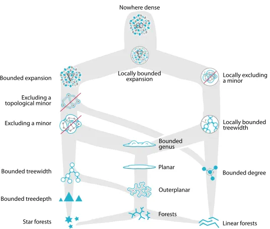
The sparse graph hierarchy is a classification system of structurally sparse graphs formally organized1 by Nešetˇril and Ossana de Mendez [74]. It organizes infiniteclassesof graphs into nested groups based on common structural properties. For example, the class of paths are a class of planar graphs as well as a class of trees. The relationships among some properties of sparse graphs are shown in Figure 2.1. We will describe classes as low or high on the hierarchy in a manner that coincides with the orientation of Figure 2.1: lower classes are more structurally restrictive. In the remainder of this section, we describe characteristics of the
1Many notions of sparsity were already defined in the literature prior to the work by Nešetˇril and Ossana de
Star forests Bounded treedepth Bounded treewidth Excluding a minor Excluding a topological minor Bounded expansion Outerplanar Planar Bounded genus Linear forests Bounded degree Locally bounded treewidth Locally excluding a minor Forests r rr ∇
∇ Locally bounded expansion Nowhere dense ∇ ∇ r ω ω
Figure 2.1An artistic rendering of the sparse graph hierarchy by Felix Reidl.
sparse graph classes on which this work is centered: bounded treedepth, excluded (toplogical) minors, bounded expansion, nowhere dense, and bounded degeneracy.
2.2.1 Treedepth
Classes of graphs withbounded treedepth [70] are relatively low on the sparse graph hierarchy, and characteristically have structure similar to that of a collection of shallow trees.
Definition 1. Atreedepth decompositionof a graph G is an injective mappingψ:V(G)→V(F),
where F is a rooted forest and uv∈E(G) =⇒ ψ(u)is an ancestor or descendant ofψ(v). Thedepth
of a treedepth decomposition is the depth of F. Thetreedepth of G, denotedtd(G)is the minimum depth of a treedepth decomposition of G.
In other words, a treedepth decomposition arranges the vertices ofGin such a way that no edge joins vertices from different branches of the tree. We can also equivalently define the treedepth using theclosureof a tree.
Definition 2. Let F be a rooted forest. Theclosureof F, denotedclos(F)is the graph whose vertex set is V(F)and vertices u,v∈ V(F)are adjacent if and only if u is an ancestor of v or v is an ancestor of u in F.
Ifψis a treedepth decomposition mappingGintoF, clos(F)contains all the possible edges
Proposition 1. The treedepth of G is equal to the minimum depth of a rooted forest F such that G⊆clos(F).
Treedepth is also closely related to a special type of graph coloring. For any subgraph H, coloringφ, and color c, if there is exactly one vertex v∈ Hsuch thatφ(v) =cwe sayc appears
uniquelyin Handv is thecenterofHwith respect toφ. A subgraph with no unique color is
said to benon-centered.
Definition 3. Acentered coloringof graph G is a vertex coloring such that every connected subgraph H has a center. We refer to the minimum number of colors needed for a centered coloring of G as its centered coloring number, denotedχcen(G).
Algorithm 1 centcolor(G,T)
Input: Graph G, treedepth decompositionT of G
Output: Canonical centered coloringφof Gwith respect toT 1: k←depth(T)
2: for allv ∈Vdo
3: φ(v)←depth(v) 4: end for
5: return φ
Algorithm 2 tddecomp(G,φ)
Input: Graph G, centered coloringφofG
Output: Canonical treedepth decompositionT of Gwith respect to φ 1: if|G|=0then
2: return ∅
3: end if
4: v←center(φ|G) 5: root(T)←v
6: for allcomponentsC∈G\ {v}do
7: T0 ←tddecomp(C,φ|C) 8: parent(root(T0))←v
9: end for
10: return T
centered coloring usingk colors by using Algorithm 1, which bijectively assigns the colors to levels of the tree and colors vertices according to their level. Likewise, given a centered coloring with k colors, we can generate a treedepth decomposition of depth at most k by choosing a centervto be the root and recursing on the components ofG\ {v}, as detailed in Algorithm 2. We refer to colorings and treedepth decompositions resulting from Algorithms 1 and 2 ascanonical. Together, these algorithms imply the treedepth and the centered coloring number of a graph are equal.
Proposition 2. [70]td(G) =χcen(G).
2.2.2 Excluded Minors
Graph minors are at the heart of structural graph theory because much of the sparse graph hierarchy can be formally characterized by the presence or absence of particular graph minors. Definition 4. Graph H is said be aminorof graph G if a series of vertex deletions, edge deletions, and edge contractions can transform G into H.
For example, the famous theorem of Wagner [101] states that the planar graphs are exactly those graphs that exclude the complete bipartite graph K3,3 and the complete graphK5 as minors. Classes thatexclude a minor, otherwise known asH-minor-free classes, generalize planar graphs and many of the other lower classes on the hierarchy; every classC in an H-minor-free class has an associated (non-empty) finite set of graphsCex such that no graphG∈ C has a minor inCex. By the celebrated Robertson and Seymour graph minor theorem [85, 86], if a class of graphsC isminor-closed—meaning that every minor of a graphG∈ Cis also a member ofC—thenC is an H-minor-free class.
This theorem can be used to prove that bounded treedepth classes are also H -minor-free. Contracting an edge corresponds to merging a vertex with an ancestor in a treedepth decomposition, which maintains the validity of the treedepth decomposition and thus does not increase the treedepth. Since a centered coloring of Gis also a centered coloring of its subgraphs, edge and vertex deletions cannot increase the treedepth either. Thus for any minor HofG, td(H)≤td(G)proving that bounded treedepth classes are minor-closed.
We can also characterize graph classes by excluding only certain types of minors. Particular focus has been paid totopological minors, which preserve topological embeddings.
Definition 5. Graph H is said to be atopological minorof graph G if a series of vertex deletions, edge deletions, and smoothings can transform G into H.
2.2.3 Bounded Expansion
Some classes that are not minor-closed are still structurally sparse in meaningful ways. Another class known asbounded expansion[71–74] can be characterized by looking at the way in which certain minors are constructed.
Definition 6. Graph H is said to be an r-shallow minorof graph G if there exist subsets V1, . . . ,V`
of V(G)such that
1. The sets V1, . . . ,V`are pairwise disjoint.
2. For each Vi there exists a vertex x∈Vi such that for all y∈Vi, the distance in G[Vi]from x to y
is at most r.
3. There is a bijectionψ:V(H)→ {V1. . .V`}such that if u,v∈ H are adjacent, then some vertex
inψ(u)is adjacent to a vertex inψ(v).
The set of all r-shallow minors of G is denoted G∇r.
In other words, ther-shallow minors are formed by contracting small diameter subgraphs into the vertices of the minor while maintaining the connectivity between the contracted subgraphs. Classes of bounded expansion limit the edge density of the r-shallow minors, allowing dense minors to be formed only when sufficiently large radius subgraphs are contracted.
Definition 7. Define thegreatest reduced average density(grad) to be
∇r(G) = max H∈G∇r
kHk |H|.
A class of graphsC is said to havebounded expansionif there exists some function f(r)such that for each G∈ C,∇r(G)≤ f(r)for all r.
Although excluding graph H as a topological minor is not in general equivalent to excluding Has a minor, an analogous definition of shallow topological minors can also be used to characterize bounded expansion classes.
Definition 8. Graph H is said to be an r-shallow topological minor of graph G if there exists U⊆V(G)and paths P1, . . . ,P` in G, where Pi =vi,1, . . . ,vi,qi such that
1. For each1≤i≤`, Pi∩U={vi,1,vi,qi}.
3. Each qisatisfies qi ≤2r+1.
4. There exist bijectionsψV :V(H)→U andψE : E(H)→ {P1, . . . ,P`}such that u,v∈ H are
adjacent if and only ifψE(uv) =Pi, v=vi,1and u =vi,qi for some i.
The set of all r-shallow topological minors of G is denoted G∇˜r.
Definition 9. Thetopological greatest reduced average density(top-grad) to be
˜
∇r(G) = max H∈G∇˜r
kHk |H|.
Proposition 3. [71] A class of graphsChas bounded expansion if and only if there exists some function f(r)such that for each G∈ C,∇˜r(G)≤ f(r)for all r.
Algorithms for classes of bounded expansion tend not to directly use the exclusion of shallow (topological) minors, but instead use a particular type of vertex coloring to identify structure. Since not all classes with bounded expansion also have bounded treedepth, we cannot assume they have centered colorings with a bounded number of colors. There is, however, a relationship between bounded expansion and a localized variant of centered colorings called p-centered colorings.
Definition 10. A p-centered coloringof graph G is a vertex coloring such that every connected subgraph H has a unique color or uses at least p colors. The minimum number of colors needed for a p-centered coloring of G is denotedχp(G).
By this definition and Algorithm 2, any set of vertices using i< p colors induces a graph whose treedepth is at mosti. These p-centered colorings give an alternative characterization of classes with bounded expansion.
Proposition 4. [71] A class of graphsC has bounded expansion if and only if for some function f(p), every graph G∈ C satisfiesχp(G)≤ f(p)for all p.
Of central importance to computing p-centered colorings efficiently are transitive fraternal augmentations (TFAs) [74]. The idea of TFAs is to augment the graph with directed arcs in order to encode local properties; to encode information about subgraphs of radiusr, we must performriterations of the algorithm. Since TFAs work with directed graphs, we first transform G into a directed acyclic graph (DAG) G~1 by orienting the edges in a way that minimizes indegree (such as using Algorithm 3 in Section 2.2.5). We then create a sequence of DAGs
~
G1 ⊆ G~2 ⊆ · · · ⊆ G~r in whichG~i+1 is formed by adding arcs between all pairs oftransitive andfraternalvertices inG~i. Verticesu,vare said to betransitiveif there is a vertexxsuch that
if they are fraternal we add either uvorvudepending on whether which choice preserves acyclicity and minimizes indegree. To obtain p-centered colorings with a bounded number of colors, we use the following two results.
Proposition 5. [71] If G belongs to a class of bounded expansion C, then for any i the maximum indegree of the ith TFA depends only onC.
Proposition 6. [71] Letσbe a topological ordering of the pth TFA,G~p. Then a greedy coloring of~Gp
overσis a(p+1)-centered coloring of G.
Proposition 5 also implies that the number of augmenting arcs in each round does not grow arbitrarily large in classes of bounded expansion, which means that the algorithm runs in time linear in the size of the graph.
Reidl introduced an alternative to TFAs calleddistance-truncated transitive fraternal augmen-tations(DTFAs) in which only the “most important” arcs are added in each round [83]. This algorithm assigns an integer labelwto each arc in~Gi. All arcsuv∈G~1receive labelw(uv) =1; arc uvis added to Gi with w(uv) = iif transitive pair u,v satisfiesw(ux) +w(xv) ≤ i and likewise ifu,vare fraternal. In this way, DTFAs shortcut paths of length at mosti. We note that every arc in theith DTFA must also be in theith TFA ofG, which means that Propositions 5 and 4 have analogous versions for DTFAs.
Proposition 7. [83] If G belongs to a class of bounded expansion C, then for any i the maximum indegree of the ith DTFA depends only onC.
Proposition 8. [83] There exists a function f such that a greedy coloring over a topological ordering of the f(p)th DTFA~Gf(p) is a p-centered coloring of G.
2.2.4 Nowhere/Somewhere Density
Nešetˇril and Ossona de Mendez usedr-shallow minors to dichotomize between structurally sparse classes and structurally dense classes.
Definition 11. A class of graphsC is said to benowhere denseif there is a function f(r)such that every graph G∈ C does not have an r-shallow clique minor of size f(r).
2.2.5 Degeneracy and Core Decompositions
The structure of graphs can also be viewed through a lens other than that of graph minors. The degeneracyof a graph can identify the presence of a dense “core” in a graph.
Definition 12. A graph G is d-degenerateif there exists an ordering of its verticesσsuch that every
vertex has at most d neighbors that precede it inσ. The smallest d for which G is d-degenerate is the
degeneracyof G and an orderingσthat witnesses this property is adegeneracy ordering.
Unlike many other structural properties such as treedepth or grad, computing the degen-eracy can be done in linear time using Algorithm 3. Reversing the order that the vertices were removed in Algorithm 3 gives a degeneracy ordering.
Algorithm 3 degeneracy(G) Input: Graph G
Output: Degeneracy ofG
1: i←0
2: while|G|>0do
3: whilethere is a vertexvof degree≤ ido
4: G←G\ {v}
5: end while
6: i←i+1
7: end while
8: return i−1
Algorithm 3 also identifies structural information on the vertex level. The core number of a vertex v is the value of i when v is removed from the graph, while the k-core of G is the subgraph induced on all vertices of core number at least k. Thus, the degeneracy can equivalently be viewed as the largest value of k for which G has a non-empty k-core. The organization of a graph into itsk-cores is known as acore decomposition.
2.3
Random Graph Models
The taxonomy of the sparse graph hierarchy provides a unique lens from which to view graphs formed by randomized processes. Arandom graph model(RGM) defines a randomized process by which a graph can be generated. One of the most basic models is the Erd˝os-Rényi random graph [33] in which the edge between any pair of the n vertices appears independently with probability p. More sophisticated processes have been devised in order to generate random data instances that match properties of real-world networks, such as their degree distributions [19] or the existence of communities [15].
2.3.1 Asymptotic Properties
While network scientists have often used random graph models to generate synthetic data on which to test algorithmic techniques, they are important to structural graph theory in a different way. Since the classification scheme on the sparse graph hierarchy relies on categorizing infinite families of graphs, there is not a way to place single networks into the hierarchy. On the other hand, random graph models can be used to define infinite families of graphs. Although many random graph models have a non-zero probability of generating any finite graph, as the size of the generated graphs grows large, certain properties may be very likely (or unlikely) to occur. Asymptotic behavior can be used to formally define “very likely”. Definition 13. A random event X is said to happenasymptotically almost surely(a.a.s.) if
lim
n→∞P[X] =1.
This allows us to say that a random graph model belongs to a particular structural class as long as it produces graphs that a.a.s. have some structural property. It has been proven, for example, that the Erd˝os-Rényi model a.a.s. has bounded degeneracy [80] but linear (and thus unbounded) treedepth [38] when the average degree is held constant, e.g., p∈O(1/n).
2.3.2 RGMs with Bounded Expansion
Perturbed Bounded Degree
Demaine et al. [27] proved that a significant generalization of the Erd˝os-Rényi model has bounded expansion a.a.s. This model, which they callperturbed bounded degreebegins with a bounded degree graph and then allows arbitrary probabilities to be assigned to each other potential edge. As long as all such probabilities are bounded by O(1/n), the model has bounded expansion.
Stochastic Block
The stochastic block modelis similar to the Erd˝os-Rényi model but also tries to simulate the existences of communities. It takes as input a partition of the vertices intor subsetsC1, . . .Cr
and anr×r probability matrix P. For verticesu∈Ci and v∈Cj, the probability that edgeuv
appears isP[i,j]. This allows the user to set higher probabilities to edges with both endpoints in a clusterCi than to edges that bridge two clusters. The proof for the perturbed bounded
degree immediately implies bounded expansion in thestochastic block modelas long as all such probabilities are bounded byO(1/n).
Chung-Lu
It is also proven in [27] that the Chung-Lu model [19] can generate graphs that a.a.s. belong to a class of bounded expansion. The Chung-Lu model produces random graphs that in expectation match a specified degree sequenceD. The structural sparsity of graphs generated by the Chung-Lu model is dependent on the proportion of vertices expected to have high degree. When this proportion decays supercubically, e.g.,O(1/d3+e), vertices have degreed,
the model has bounded expansion a.a.s. If the decay is subcubic e.g.Ω(1/d3−e), the graphs
generated are in a somewhere dense class a.a.s., while a cubic decay implies the graphs will a.a.s. belong to a nowhere dense class with unbounded expansion.
The Chung-Lu model can easily match heavy-tailed degree distributions commonly found in real-world networks but struggles to match other properties like clustering. To remedy this, a variant of the model addshouseholds, meaning that it generates the prescribed degree distribution and then expands each vertex into a small subgraph with high clustering, such as a clique. Provided that the households have constant size with respect ton, the above results are still applicable to the household variant.
“copies”). For most of the networks, the number of colors used in thep-centered coloring in the real data was within or below the range of number of colors for the corresponding synthetic data sets. Since bounded p-centered coloring numbers imply bounded expansion, the authors concluded that these networks indeed had structure consistent with bounded expansion.
Random Intersection
In other research [34] therandom intersection modelhas been shown to produce graphs that a.a.s. belong to classes of bounded expansion under certain conditions. The random intersection model begins with two sets of verticesVand Aand creates a bipartite graph by adding edges betweenV andAuniformly at random with probability p. For each pair of vertices u,v∈V, the edge uv is added if u and v have a common neighbor in A. At the conclusion of this process, Ais discarded and Vand its edges are returned. This process simulates a network of entities whose connectivities are based on mutual attributes e.g. students who have taken a common class. When the probability of each random edge is bounded byO(1/|V|1+e), the
random intersection model a.a.s. has bounded expansion.
2.4
Parameterized Complexity
Having introduced the graph theoretical concepts that form the foundation of this work, we now continue to the concepts from complexity theory. Though all NP-complete problems are “equally hard”, additional information can make some problems easier to solve. The field of parameterized complexityformalizes this notion with the definitions of additional subclasses of NP; in this work we consider the classes XP and FPT (fixed parameter tractable).
Definition 14. Given an input of size n and a positive integer parameter k, an algorithm belongs to the class XP if its time complexity is O(nf(k))for some computable function f .
Definition 15. Given an input of size n and a positive integer parameter k, an algorithm belongs to the class FPT if its time complexity is O(f(k)·nc)for some computable function f and constant c.
Algorithms in XP and FPT can run efficiently when the parameterkis small, but devolve into super-polynomial algorithms whenkis not a constant.
2.4.1 Relationship to Graph Structure
Parameterized complexity is strongly intertwined with structural graph theory because the structural characteristics of sparse classes can be exploited to solve otherwise intractable prob-lems more efficiently. For some classes, the connection between structure and parameterized algorithms is straightforward. Classes of bounded treedepth, for instance, are characterized as having treedepths that do not grow with the size of graphs in the class. An algorithm that uses the treedepth as the integer parameter k would have the value of f(k) bounded by a constant independent ofnfor all graphs in the class and the asymptotic complexity will be simplyO(nc)for some constantc. The bounded treedepth property is often exploited by such an algorithm by performing some brute force computation over some set of inputs exponential in the treedepth. For example, it might take paths from leaves to the root of the treedepth decomposition and find the optimum value of a function over all 2td(G) subsets of vertices on each path. Since the treedepth decomposition restricts the ways these root paths overlap, function values from different root paths could be combined using dynamic programming, ultimately leading to computing that function for the entire graph.
Exploiting the structural properties of other classes is not always as obvious. The absence of certain (r-shallow) minors does not immediately translate into an integer parameter necessary for a parameterized algorithm and hence algorithms exploiting excluding a minor and bounded expansion require more clever tricks. As will be discussed at length in Chapter 4, some algorithms for classes of bounded expansion make extensive use of p-centered colorings. Since bounded expansion classes admitp-centered colorings with a number of colors independent of n, enumerating the subgraphs induced on all subsets ofp−1 colors can be done inO∗(χp(G)p)
time. Since each of these subgraphs has bounded treedepth, algorithms parameterized by treedepth can be run on each of the subgraphs and then their results can be combined to generate a solution for the entire graph.
2.4.2 Parameterized Lower Bounds
It can be useful to determine when a fixed-parameter tractable algorithm has reached “best possible” asymptotic dependence on the parameter. One method for establishing a parameter-ized algorithm is by showing faster algorithms violate theexponential time hypothesis(ETH), which is a complexity-theoretical conjecture relating to the hardness of k-SAT.
Input: Boolean formula Φink-CNF form
Conjecture 1([47]). There is no algorithm for k-SATwhose worst-case time complexity is2o(n)for a formula with n variables.
The ETH is a stronger assumption than P 6= NP since the latter would not exclude, for example, an algorithm fork-SAT running inO(2
√
n)time. To use the ETH to derive a lower
CHAPTER
3
LOCALLY ESTIMATING CORE
NUMBERS
Summary
“Central” vertices in a graph tend to be more critical in the spread of information or disease and play an important role in clustering/community formation. Identifying such “core” vertices has recently received additional attention in the context of network experiments, which analyze the response when a random subset of vertices are exposed to a treatment (e.g. inoculation, free product samples, etc). This notion of centrality can be expressed by the core numbers of the vertices. Existing algorithms for computing the core number of a vertex require the entire graph as input, an unrealistic scenario in many real world applications. Moreover, in the context of network experiments, the subgraph induced by the treated vertices is only known in a probabilistic sense. We answer Research Question 1 by introducing a method for estimating the core number based only on the properties of the graph within a region of radiusδaround
the vertex, and prove an asymptotic error bound on random graphs. Further, we empirically validate the accuracy of our estimator for small values ofδon a representative corpus of real
3.1
Introduction
In a graph modeling complex interactions between data instances, the connectivity of the vertices often yields useful insights about the properties of the represented entities. For example, in a social network, it is important to distinguish between a person who is a member of a relatively large, tight-knit community, and a person who exists on the periphery without much involvement with any cohesive communities. This type of connectivity is often not well-correlated with the vertex degree (raw number of connections), leading to the introduction of several more sophisticated metrics. Here, we focus on thecore number[6]. To build intuition, consider the setting of a graph representing friendships in a social network – the vertices with large core numbers form a set where people tend to have many common friends, whereas the subset of vertices with small core numbers form a group where most people do not know one another. The applications of core numbers are numerous, well studied, and permeate a variety of domains, such as community detection [39, 64], virus propagation [52], data pruning [4], and graph visualization [2].
Existing algorithms for computing core numbers run in linear time with respect to the number of vertices and edges of the graph [6], but require the entire graph as input and simultaneously calculate the core number for every vertex. There are a number of scenarios in which current approaches are insufficient. First, one might only be concerned with the properties of a small subset of query vertices1. If the query vertices constitute a small fraction of the entire graph, it would be much more time- and memory-efficient to locally estimate the core numbers of those specific vertices rather than using the global algorithm, regardless of the fact that it is linear. Second, the entire graph may be unknown and/or infeasible to obtain due to scale, privacy, or business strategy reasons. For example, suppose one wanted to investigate patterns of phone calls between cell phone users. It would be possible to contact a small set of people and ask them to voluntarily log their calls for one month. However, without access to the telecommunication companies’ private records, expanding the domain to the national or global level would not be possible. Finally, current methods for determining core numbers cannot be applied to solve problems in the domain of network experimentation, as we describe below.
Anetwork treatment experimentis a randomized experiment in which subjects are divided into two groups: those receiving treatment and those receiving none (or a placebo). Network treatments differ from other randomized experiments in that the effects of the treatment (or lack thereof) on a given subject are assumed to be dependent on the experiences of other subjects in the experiment. Randomly assigning subjects into two groups (treated versus untreated) is
1For example, vertices which have some common metadata (e.g. age, physical location, etc.) of interest to the
equivalent to randomly partitioning the vertices of a graph into two sets. Previous work has given methods to calculate degree probabilities of a randomly partitioned graph [99], but an analogous algorithm for the core numbers is an open problem. Given the results of Kitsak et al. on the importance of core numbers in spreading information [52], an algorithm to predict the likelihood of a given subject having a large core number would help researchers better understand the impact of their experimental design. For example, researchers conducting market testing on a product that relies on social interaction (such as a new social networking site, online game, etc.) would have a greater ability to see whether early access to their product will generate widespread excitement among the test subjects. Additionally, if certain groups of vertices (say, females participating in the experiment) are more likely to be core exposed than the others, we can reduce the bias of the estimate of the treatment effect by upweighting the probability that underrepresented vertices (males) are treated.
All of the challenges mentioned above and Research Question 1 could be addressed by estimating the core number of a vertex based on local graph properties. The existence of an accurate non-global estimator is intuitively well-grounded, as it has been shown that addition and deletion of edges can only affect the core numbers of a limited subset of vertices [87]. This suggests that in spite of the fact that computing core numbers exactly requires knowledge of the whole graph, the core number of a given vertex may often depend on a much smaller subgraph. Moreover, even if a core number estimate has a small error, it may still be useful in applications. In particular, it is often sufficient to delineate between vertices with a “large” core number and those with a “small” core number. That is to say, while a vertex in the 50-core is substantially more well-connected than one in the 2-core, it may be functionally identical to a vertex in the 51-core in downstream analysis.
3.2
Related Work
The basic k-core decomposition algorithm has been tailored to meet additional constraints. Montressor et al. [67] and Jakma et al. [48] proposed methods by which the core decomposition could be computed in parallel. Li et al. [87] and, later, Saríyüce et al. [57] described ways to update the core numbers of vertices in a dynamic graph without recomputing the full core decomposition each time a vertex or edge is added. Finally, Cheng et al. [17] gave an alternate implementation of the core decomposition for systems with insufficient memory to store the entire graph at once.
3.3
Local Estimation
In order to estimate core numbers efficiently without knowledge of the entire graph, we will restrict the domain of our algorithms to a localized subset around a vertex:
Definition 16. Theδ-neighborhoodof a vertex v, denoted Nδ(v), is the set of vertices at distance2
at mostδfrom v.
The estimation algorithms will vary the size of their input by allowing δ to range from
zero to∆, thediameterofG(the maximum distance among all pairs of vertices).
3.3.1 Neighborhood-based Estimation
A relatively naïve approach to local estimation would be to compute a core decomposition of the subgraph ofGinduced on theδ-neighborhood ofvand use the resulting core number of v
as the estimate:
Definition 17. Let theinduced estimator,k˘δ(v), be the core number of v in G[Nδ(v)].
By increasingδ, the induced subgraph captures a progressively larger fraction of the graph,
improving the estimate until ˘kδ(v) = k(v) (which is guaranteed to happen at δ = ∆, but
could happen for significantly smaller δ). Note that whenδ = 1, the estimator will only be
close to the core number if the neighbors ofvare highly interconnected (so there is a subtle relationship to clustering coefficient).
Lemma 1. Let G= (V,E)be a graph. For all v∈V, 0=k˘0(v)≤k˘1(v)≤ · · · ≤k˘∆(v) =k(v)
Proof. First we will establish the boundary conditions on our inequality. Because N∆(v) =G, ˘
k∆(v) = k(v). Since N0(v) = {v}, ˘k0 = 0. Additionally, for all δ ∈ [1,∆], Nδ−1(v) ⊆ Nδ(v).
This implies that for all u ∈ V, the degree of u in the subgraph induced by the (δ−
1)-neighborhood ofv can be no greater than the degree ofuin theδ-neighborhood ofv. Thus v
cannot participate in a deeper core with respect to the(δ−1)-neighborhood than it does with
respect to theδ-neighborhood, which makes ˘kδ−1≤k˘δ.
In order to make a more sophisticated estimation, let us consider the information gained asδincreases. Atδ=0, we assume that d(v)is known. Because thek-core requires all vertices
to have minimum degree k, k(v) can not be greater than d(v). Thus, d(v) itself can be an estimate ofk(v). Expanding out toδ=1 allows information aboutv’s immediate neighbors
to be utilized. Suppose the core numbers of the neighbors ofv were known. It would then be possible to computek(v)precisely using the following two lemmas (previously shown by Montresor et al):
Lemma 2([67]). A vertex v is in the j-core of a graph G if and only if v has at least j neighbors in the j-core.
We now give a closed-form algebraic expression for the largest jsatisfying Lemma 2. Lemma 3([67]). Let u1,u2, . . . be the k-ordered neighbors of v. Then
k(v) = max
1≤i≤d(v)(min(k(ui),d(v)−i+1)).
Proof. By the definition of core number and Lemma 2, k(v) is the largestj in 0 ≤ j ≤ d(v) so that v has at least j neighbors with core number at least j. For each ui (1 ≤ i ≤ d(v)),
v has d(v)−i+1 neighbors with core numbers at least k(ui), since k(ui) ≤ k(ui+1). If k(ui)≤ d(v)−i+1,vhas at leastk(ui)neighbors in thek(ui)-core. Otherwise,vhas at least
d(v)−i+1 neighbors in the(d(v)−i+1)-core. This shows that the core number ofvmust be at least the minimum ofk(ui)andd(v)−i+1 for everyi(and thus the maximum overi). Equality follows easily by contradiction.
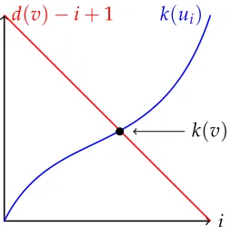
Note thatk(v)is the maximum value of the minimum of two functions ofi:k(ui)andd(v)−
i+1. With respect toi,k(ui)is monotonically non-decreasing andd(v)−i+1 is monotonically
decreasing. From a geometric perspective, then, the maximum of their minimums occurs at the intersection of the curvesk(ui)andd(v)−i+1 (as stylized in Figure 3.1).
i
d(v)−i+1 k(ui)
k(v)
Figure 3.1The core numberk(v)is they-value at intersection of two functions.
Theorem 1 ([17]). Let G = (V,E) be a graph, v ∈ V, and ψ any function satisfying ψ(u) ≥
k(u)∀u∈ V. Let v’s neighbors beψ-ordered. Then
k(v)≤ max
1≤i≤d(v)(min(ψ
(ui),d(v)−i+1)).
Proof. Substitutingψ(ui)fork(ui)in the expression from Lemma 3 can only increase the right
hand side, giving an upper bound onk(v).
We base our second estimator on the idea of incorporating iterative upper bounds on the core numbers of a vertex’s neighbors:
Definition 18. Let thepropagating estimator,kˆδ, be the estimator of k(v)given by the recurrence
ˆ kδ(v) =
max 1≤i≤d(v)
min(kˆδ−1(ui),d(v)−i+1)
ifδ>0
d(v) ifδ=0
where u1,u2, . . . are thekˆδ−1-ordered neighbors of v.
Pseudocode for computing ˆkδ(v)is given in Algorithm 4. Essentially, Algorithm 4 first
computes the coarsest upper bound (ˆk0) for those vertices at distance at mostδfromv. Those
estimates are used in conjunction with Theorem 1 to compute a slightly finer upper bound, ˆ
k1, for those vertices at distance at most δ−1 from v. This process “propagates” inwards
towardsvuntil its immediate neighbors have ˆkδ−1 values, which are used as the upper bounds in formulating ˆkδ(v). The computational complexity of finding ˆkδ is linear in the product of δ and the number of edges in Nδ(v)(see Theorem 2). Since Algorithm 3 is also linear with
respect to the number of edges in the graph, the computational complexity of computing ˆkδ is
Algorithm 4 prop_estimator(v,δ)
Input: Vertexv, distanceδ
Output: Propagating core number estimator ofvat distanceδ, i.e., ˆkδ(v) 1: ifδ=0then
2: return d(v)
3: else
4: foru∈ N1(v)do
5: kˆδ−1(u)←prop_estimator(u,δ−1)
6: end for
7: kˆδ(v)←d(v)
8: fori∈ {1, . . . ,|N1(v)|}do
9: ui ←vertex inN1(v)theith smallest value of ˆkδ−1 10: j←min(kˆδ−1(ui),d(v)−i+1)
11: ifj> kˆδ(v)then 12: kˆδ(v)←j 13: end if
14: end for
15: return kˆδ(v) 16: end if
Theorem 2. For a given vertex u,kˆδ(u)can be computed in O(δ· |Eδ(u)|)time using Algorithm 4,
where Eδ(u)is the edge set of G[Nδ(u)].
Proof. Fix δ ∈ {1, 2, . . .} and u ∈ V. Assume ∀u0 ∈ N1(u), ˆkδ−1(u
0) is known. Since ˆk
δ can
only take integer values in the interval [0, maxv∈Vd(v)], the sorting (line 9) can be done in
O(d(u)) time using a bucket sort. Once sorted, each neighbor of u is visited once (line 8) to find the minimum, which can also be done inO(d(u))time. Thus computing ˆkδ(u)from
{kˆδ−1(u0)|u0 ∈ N1(u)}has complexityO(d(u)).
Using dynamic programming, we can compute and store ˆk1(w) ∀w ∈ Nδ−1(v), which
in turn can be used to compute ˆk2(w) ∀w ∈ Nδ−2(v), and so on (through δ−1 iterations) until we have computed ˆkδ(v). The jth such iteration requires ∑u∈Nδ−jO(d(u)) =O(Eδ−j(v)) operations. SinceNδ−1⊆ Nδ, the total running time isO(δ· |Eδ|).
Unlike ˘kδ(v), the estimate ˆkδ(v)is a decreasing upper bound onk(v)asδincreases:
Theorem 3. ∀v∈ V, k(v)≤kˆδ(v)≤kˆδ−1(v)· · · ≤ˆk1(v)≤ ˆk0(v) =d(v)for anyδ ≥1.
Proof. We first prove that k(v)≤kˆδ(v)for all δ≥ 0 by induction onδ. The base casek(v)≤
ˆ
k0(v) = d(v)holds, since core number is always bounded by degree. Assumek(v)≤ kˆδ(v).
Then ˆkδ is an upper bound ψ as in Theorem 1, and substituting the right hand side with
v
w1 w2
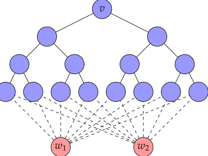
Figure 3.2T2,4is in blue.T2,40 isT2,4plusw1,w2(red), and the dashed edges.
We now prove that ˆkj+1(v)≤ kˆj(v)for allj≥0 and∀v∈V by induction onj. Combining
Definition 18 with Lemma 3, we see that ˆkδ(v) is the maximum of the minimum of the
functions ˆkδ−1(ui) and d(v)−i+1 for 1 ≤ i ≤ d(v). Since the maximum of d(v)−i+1 is
d(v), ˆkδ(v)≤d(v). Because ˆk0(v) =d(v)the base case ˆk1(v)≤ kˆ0(v)is satisfied. Suppose that
for somej≥0, ˆkj(v)≤kˆj−1(v)for allv∈ V. By Theorem 1,vhas at least ˆkj(v)neighbors that
satisfy ˆkj−1(u) ≥ kˆj(v)for u ∈ N1(v). Each suchu also satisfies ˆkj(u) ≤ kˆj−1(u), meaning v can have no more than ˆkj(v)neighbors that satisfy ˆkj(u)≥kˆj(v). Thus ˆkj+1(v)≤kˆj(v).
3.3.2 Structures Leading to Error
One natural question is whether either ˆkδ or ˘kδ has bounded error (is a constant-factor
approximation of the core number). Unfortunately, there are extremal constructions forcing unbounded error for both estimators; both are based on Tj,`, the complete j-ary tree with ` levels (labeled so that levelihasji−1 vertices), rooted at a vertexv(Figure 3.2).
Lemma 4. For all integersδ≥0, x ≥1, there exists a graph G and vertex v so that
ˆ
kδ(v)−k(v) =x−1.
Proof. First note that sinceTj,` is a tree, it is 1-degenerate. We show that the root vertexvhas ˆkδ
estimators with unbounded error. For any vertexuwith level numberiin[2,`−δ−1], every
vertex not equal tovinu’sδ-neighborhood has degreej+1. As a result,d(u) =kˆ1(u) =· · · = ˆ
ki−1= j+1, and ˆki = · · ·= kˆδ = j(sincevhas degree jand will have propagated inwards).
Lemma 5. For all integersδ≥0, x ≥1, there exists a graph G and vertex v so that
˘
kδ(v)−k(v) =x−1.
Proof. Consider the graph Tj0,` created by adding vertices w1, . . . ,wj toTj,` connected to the leaves ofTj,` as apices (see Figure 3.2). Then the rootv is the vertex of minimum degree inTj0,` and has core number j. Any induced subgraph ofTj0,` that does not include at least onewi is a
tree, making it 1-degenerate. Thusk(v)−k˘δ(v) = j−1 whenever`≥ δ+1.
Note that in Tj,`, ˘kδ(v) = k(v) for any δ > 0. Likewise, in T
0
j,`, ˆkδ(v) = k(v) for any δ ≥0. Despite the fact that the errors of both estimators can theoretically be arbitrarily large,
structures causing egregious errors (like Tj,` and Tj0,`) are unlikely to occur in real world networks; we provide evidence to support this claim in the next sections.
3.3.3 Expected Behavior on Random Graphs
In order to better understand the errors generated when approximating core number with ˆkδ,
we analyze its behavior on Erd˝os-Rényi random graphs. To avoid confusion, we useG(n,p) to denote the set of all Erd˝os-Rényi random graphs with n vertices and edge probability p and G(n,p) for a specific instance. Since all graphs on n vertices occur in G(n,p) with non-zero probability (when p∈(0, 1)), analysis typically focuses on whether a graph property is very likely (or unlikely) to occur as the size of an Erd˝os-Rényi random graph grows large. In keeping with prior work ([49, 62, 80]), we assume the average degree is fixed, letting (n−1)p= d¯, a constant.
Specifically, we focus our attention on the growth of the error term ˆk1(v)−k(v)asn→∞by deriving probabilistic expressions for ˆk1(v)andk(v)for any v∈G(n,p), then demonstrating how each term grows withncompared to a function inω(1)(recall a function f(n)isω(1)if
limn→∞ f(1n) =0).
Theorem 4. Supposee(n)isω(1). Then for any v∈ G(n,p),kˆ1(v)−k(v)is O(e(n))a.a.s.
Proof. Fix a vertex v, and let S>κ, S<κ, and S=κ be defined to be the subsets of N1(v)with
vertices of degree greater than, equal to, or less thanκ, respectively. We first evaluateP[kˆ1(v) =
κ|d(v) =d]. By Definition 18, if ˆk1(v) =κ,vhas at leastκ neighborsuwith ˆk0(u)≥κbut less
thanκ+1 with ˆk0(u)≥κ+1 (or else ˆk1(v)>κ). Therefore, ˆk1(v) =κimplies|S>κ| ≤κand
|S=κ|+|S>κ| ≥κ, and
P[kˆ1(v) =κ|d(v) =d] =
κ
∑
i=0
d−κ
∑
j=0 d!
where x=d−i−j.
Asntends to infinity, the probability that any two neighbors ofvhave an edge between them approaches 0. Therefore, the degrees ofv’s neighbors can be treated as independent, identical distributions in the limit. Sincenis large and ¯dis fixed, this distribution is asymptoti-cally Poisson with mean ¯d. Ifζλ(k)andZλ(k)denote the Poisson probability mass function
and cumulative distribution function, respectively, with meanλ(evaluated at k), then:
P[kˆ1(v) =κ|d(v) =d] = κ
∑
i=0
d−κ
∑
j=0 d!
i!j!x!(1−Zd¯(κ−1))
iZ
¯
d(κ−2)jζd¯(κ−1)x. (3.1)
By computing Equation 3.1 at each value of d for which κ is a possible value for the core
number, we have:
P[kˆ1(v) =κ] = n−1
∑
d=κ
ζd¯(d)·P[kˆ1(v) =κ|d(v) =d]. (3.2)
Pittel et al. [80] demonstrated that in G(n,p), the proportion of vertices in the k-core is a.a.s. a function of ¯d but not of n. Moreover, for any vertex v, k(v) is a.a.s. bounded by a constant (equivalently, inΘ(1)). If ˆk1(v)were also bounded by a constant, then the error term ˆ
k1(v)−k(v)would be a.a.s.O(1). However, since the Poisson random variables in Equations 3.1 and 3.2 are only parameterized by ¯d and not byn, the proportion of vertices inG(n,p) with ˆk1= κis a.a.s. convergent to some non-zero constant. Thus, the probability of having an
arbitrarily large value of ˆk1 does not vanish asngrows large for a fixed (constant)κ.
Letκ be a function ofninω(1). By Stirling’s approximation of the factorial,
ζd¯(κ)≈ e
−d¯ √
2πκ
ed¯
κ κ
.
Then as n grows large, ζd¯(κ) → 0 and Zd¯(κ) → 1. In Equation 3.1, the probability that a
neighboruof vertexvhas degree at leastκ(that is, u∈S>κ∪S=κ) is asymptotically zero, and
consequentlyP[kˆ1(v) =κ]also vanishes in the limit. This implies that a.a.s.P[kˆ1(v) = κ]∈
O(e(n))for any error functione(n)∈ω(1). Using the result of [80] thatk(v)∈Θ(1), we have
a.a.s. ˆk1(v)−k(v)∈O(e(n)).
3.4
Experimental Results
In the previous section, the behavior of the propagating estimator ˆkδ was analyzed from a
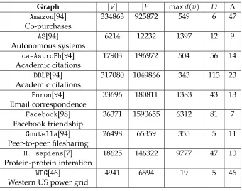
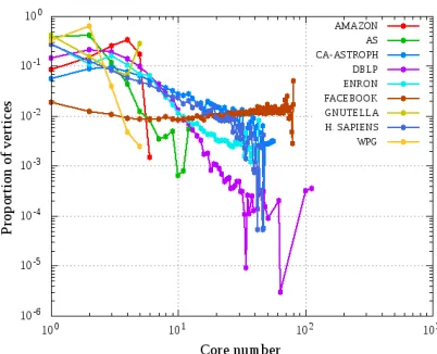
Table 3.1Summary statistics for real-world graphs used in evaluating local core estimators.
Graph |V| |E| maxd(v) D ∆
Amazon[94] 334863 925872 549 6 47 Co-purchases
AS[94] 6214 12232 1397 12 9
Autonomous systems
ca-AstroPh[94] 17903 196972 504 56 14 Academic citations
DBLP[94] 317080 1049866 343 113 23
Academic citations
Enron[94] 33696 180811 1383 43 13 Email correspondence
Facebook[98] 36371 1590655 6312 81 7 Facebook friendship
Gnutella[94] 26498 65359 355 5 11 Peer-to-peer filesharing
H. sapiens[7] 18625 146322 9777 47 10 Protein-protein interation
WPG[46] 4941 6594 19 5 46
Western US power grid
3.4.1 Methods
The estimators ˆkδ and ˘kδ were evaluated on nine real-world graphs which cover a variety of
domains and are structurally dissimilar. The graphs vary in size, density, core structure, and diameter (see Table 3.1 and Figure 3.3).
We computed the core numberk(v), as well as the values of ˆkδ(v)and ˘kδ(v)for each vertex,
letting δ vary from 0 to ∆. To compare the accuracy of the estimators among vertices, we
normalize by the true core number at each vertex. We refer to this metric as thecore number estimate ratio. When the estimator (ˆkδ or ˘kδ) is exactly equal to the core number, the core
number estimate ratio is 1, itsoptimalvalue. Since ˆkδ is an upper bound onk, its core number
estimate ratio is always at least one and becomesless optimalthe larger it gets; the opposite is true for ˘kδ, a lower bound.
3.4.2 Results
We first turn our attention to how often the estimators achieve optimal core number estimate ratios. Figure 3.4 shows how the proportion of vertices with ratio one grows asδ increases
from zero to four. In all the graphs, the core number estimate ratio for ˆkδ is optimal at least as
Figure 3.3Core number distribution for the real world networks in Table 3.1.
ratios is large in all the graphs (often upwards of 90%). While the propagating estimator does not have as pronounced of an advantage over the induced estimator whenδ=2, the number
of vertices with optimal ˆkδ estimate ratios still grows noticeably.
We also examined the distribution of core number estimate ratios among those vertices where the estimate was not exact. The change in this distribution over the range δ = 1 to δ =4 is shown in Figure 3.5, demonstrating that not only are the sub-optimal estimates closely
centered around 1, but also that increasingδcan significantly decrease the size of the “tail” of
the distribution (thereby improving the core number estimates of those vertices with the least optimal ratios).
Although Figures 3.4 and 3.5 suggest that ˆkδ and ˘kδ can accurately estimate the core
numbers in real world graphs using only knowledge of theδ-neighborhood with a small value
ofδ, it is important to understand how the size of theδ-neighborhood impacts the behavior of
the estimates. The purpose of having a localized estimate is to reduce the size of the input needed to compute the core number of a vertex. If the averageδ-neighborhood encompasses
most of the graph, then not only is this purpose defeated, but we also may not be able to judge whether the accuracy of the localized estimates is only due to having knowledge of the entire graph (as opposed to any theoretical merits of the algorithms themselves). The mean and variance of the proportion of vertices in theδ-neighborhood is shown in Table 3.2. The rate of
growth ofδ-neighborhood sizes varies significantly among the nine graphs, which suggests
that picking a value ofδ to maintain appropriately smallδ-neighborhoods is highly dependent
on the structure of the graph. Nonetheless, the average size of theδneighborhood is below
ten percent of the entire graph for all datasets atδ =1 and in all but one (namelyFacebook,
(a)Amazon (b)AS (c)ca-AstroPh
(d)DBLP (e)Enron (f)Facebook
(g)Gnutella (h)H. sapiens (i)WPG
Another natural way to measure the relative amount of information in the δ-neighborhood
is to normalize by the diameter∆. Figure 3.6 shows that the average proportion of vertices in theδ-neighborhood is approximately uniform in all graphs whenδis expressed as a fraction
of∆. In particular, there is a significant increase in the rate of growth of theδ-neighborhood
size occurring when δ is approximately 20% of the diameter. Thus, as one might expect,
(a)Amazon (b)AS (c)ca-AstroPh
(d)DBLP (e)Enron (f)Facebook
(g)Gnutella (h)H. sapiens (i)WPG
Table 3.2Proportion of vertices inNδ. Values less than .01 rounded to 0.
δ=1 δ =2 δ =3 δ =4
Graph Avg. Var. Avg. Var. Avg. Var. Avg. Var.
Amazon 0 0 0 0 0 0 0 0
AS 0 0 .09 .01 .44 .07 .82 .04 ca-AstroPh 0 0 .03 0 .25 .04 .66 .06
DBLP 0 0 0 0 0 0 .03 0
Enron 0 0 .03 0 .28 .04 .74 .06 Facebook 0 0 .21 0.03 0.89 0.02 1 0
Gnutella 0 0 0 0 .02 0 .15 .02
H. sapiens 0 0 0.31 0.07 0.81 0.04 0.98 0
WPG 0 0 0 0 0 0 .01 0
neighborhood-based core number estimates seem most appropriate whenδis a small fraction
of the diameter.
(a)Amazon (b)AS (c)ca-AstroPh
(d)DBLP (e)Enron (f)Facebook
(g)Gnutella (h)H. sapiens (i)WPG
To see the effect of this normalized setting on accuracy, consider Figure 3.7. After nor-malizingδby the diameter, the variation between graphs is less pronounced. Even whenδis
small compared to∆, the optimum core number estimate ratio can be achieved. It is worthy to note thatFacebookis a stark exception in which a significant proportion of vertices cannot achieve an optimal core number estimate ratio even whenδ=∆. This graph has many vertices
withd(v)k(v)and a small diameter. Thus, many vertices have very inaccurate ˆk0-values, which propagate inwards and remain uncorrected due to the small number of refinements performed on the estimate. Ultimately, we conclude that ˆkδ best achieves its goal of accurately
estimating the core number using only a small local section of the graph when the graph has a large diameter and the ratioδ/∆is small (e.g. less than 0.2).
3.5
Network Treatment
We now turn to the domain of network experiments and use the ˆkδ estimator to address an
open problem given in [99].
3.5.1 Problem Statement
Recall from the introduction that anetwork treatment experimentis a random experiment in which some subjects are given a treatment and the rest are not. It differs from other experiments in that the effects of the treatment are assumed to be dependent on interactions between subjects, which can be modeled by a graph. The general goal is to measure the subjects’ experiences in a hypothetical universe where the entire graph is treated by observing the experience of the subject when only some of the graph is treated. Ugander et al. [99] focused on local properties of the vertices to compare these two scenarios. In particular, they identified two useful ways to concretely measure the experience of a subject via graph properties: Definition 19([99]). A vertex v experiencesabsolutek-degree exposureif v and at least k of v’s neighbors receive treatment.
Definition 20([99]). A vertex v experi

![Figure 3.9 P[X(d)κ ] − P[ ˆXκ] for the W P Ggraph at p = 0.25. Vertices with P[X(d)κ (v)] = 0 are omitted.](https://thumb-us.123doks.com/thumbv2/123dok_us/1182815.1148668/50.612.99.538.91.278/figure-k-p-xk-w-ggraph-vertices-omitted.webp)
