Design of a Parallel Self-Timed Adder using Recursive Approach
Nalamala Ramya
, B. Baloji Naik , K. Amit Bindaj
[email protected],[email protected]
1MTECH, Sai Tirumala NVR Engineering College, Jonnalagadda, Narasaraopet, Guntur, Andhra Pradesh, India 2Associate Professor, Dept of ECE, Sai Tirumala NVR Engineering College, Jonnalagadda, Narasaraopet, Guntur, Andhra
Pradesh, India
3HOD, Dept of ECE, Sai Tirumala NVR Engineering College, Jonnalagadda, Narasaraopet, Guntur, Andhra Pradesh, India
Abstract:
Many pipelined adaptive signalprocessing systems are subject to a trade-off between throughput and signal processing performance incurred by the pipelined adaptation feedback loops. In the conventional synchronous design regime, such throughput/performance trade-off is typically fixed since the pipeline depth is usually determined in the design phase and remains unchanged in the run time. With this motivation, we propose to apply self-timed pipeline, an alternative to synchronous pipeline, to implement the pipelined adaptive signal processing systems, in which the pipeline depth can be dynamically changed to realize run-time configurable throughput/performance trade-offs. Based on a well-known high speed self-timed pipeline style, we developed architecture and circuit level design techniques to implement the self-timed pipelined adaptation feedback loop with configurable pipeline depth.
The data transfer rate in hard disk varies as the read head moves among tracks with different distance from the center of the disk platter. By adjusting the pipeline depth on-the-fly, the DLMS equalizer can dynamically track the best equalization performance allowed by the varying data transfer rates. Simulation result shows a significant performance improvement compared with its synchronous counterpart.
Keywords: Manchester coding, Encoder, Decoder,
NRZ, Moore’s law, UART, clock frequency.
I. INTRODUCTION
Over the last two decades, adaptive signal processing has developed into a self-contained field [1], [2] that finds wide range of real-life applications
such as adaptive equalization, noise and echo cancellation, linear predictive coding, and adaptive beam-forming. Adaptive signal processing algorithms are characterized by their recursive operations for realizing algorithmic self-designing/adaptation.
To realize high-throughput VLSI implementation of adaptive signal processing algorithms, architecture-level technique pipelining is typically used [3]. Pipelined adaptive signal processing systems are essentially subject to a trade-off between system throughput and signal processing performance, i.e., deeper pipelined adaptation feedback loop can realize higher throughput, but the delayed feedback will incur larger performance degradation. It should be pointed out that, for other recursive algorithms such as infinite impulse response (IIR) filtering and Viterbi algorithm, direct pipelining may simply ruin their functionality and appropriate algorithm-level modification is required for the use of pipelining.
Self-timed pipeline [4], [5] works in a different way from its synchronous counterpart. Without a common and discrete notion of time, self-timed pipeline relies on the handshake between components to perform the synchronization and communication. Each distinct data propagating through a self timed pipeline is conventionally called a token. The pipeline depth of a self-timed pipeline simply equals the number of tokens present in the pipeline at the same time. Hence, we can dynamically configure the pipeline depth by controlling the number of tokens present in the pipeline. This property of self-timed pipeline has been exploited in the design of a mixed synchronous-asynchronous FIR filter that can support variable latency (in terms of clock cycles) [6] and power management of an embedded, single-issue processor [7].
In pipelined adaptive signal processing systems, the pipeline depth of the adaptation feedback loops is the key to tune the inherent tradeoff between throughput and signal processing performance. This directly motivates us to apply self-timed pipeline for the implementation of adaptive signal processing systems to realize gracefully configurable throughput/performance tradeoff. This can be leveraged to improve the overall system performance in many circumstances. For example, for adaptive signal processing systems with variable data rate, we can dynamically adjust the pipeline depth to the minimum allowable value according to the current data rate to realize the best signal processing performance. Although the basic idea of the above design approach is simple and intuitive, how to implement it in the real systems involves the following three critical design issues:
1) What type of self-timed pipeline structure should be used? Clearly, to justify the practicality of this design approach, the employed self-timed pipeline must be able to support the same (or comparable) throughput as its synchronous counterpart when they have the same pipeline depth. This means that the recursive self-timed pipeline data path should have the same (or comparable) propagation delay as its synchronous counterpart. This is a very strict requirement since most self-timed
pipeline design schemes involve extra delay overhead for realizing self-timed handshake and have the longer latency than their synchronous counterparts, although they can support very fine-grain pipeline to realize high throughput. In this work, we propose to use the well-known Ted William’s high-speed self-timed pipeline [4], [8] because of its zero delay-overhead feature (i.e., no extra handshake delay is incurred when data propagate through the pipeline). Hence the zero-delay-overhead pipeline can achieve the same latency performance as its synchronous counterpart.
2) How to realize the self-timed data flow synchronization in the recursive adaptation loop? In self-timed data path, synchronization of parallel computational threads relies on forks and joins, where fork refers to a stage with one input channel and multiple output channels and join refers to a stage with multiple input channels and a single output channel. The recursive adaptation loop of adaptive signal processing algorithms contains many forks and joins. However, like many other self-timed pipeline styles, the zero-delay-overhead self-timed pipeline was initially proposed for linear datapath (i.e., without forks and joins). Therefore, it must be appropriately modified to support forks and joins.
3) How to realize run-time addition/removal of tokens in order to change the pipeline depth? In a feed forward only data path, the pipeline depth can be readily changed by adjusting the input data rate. However, as we will show later, it is not trivial to change the pipeline depth in recursive adaptation loops. We have to design some special circuit elements that can be placed on the recursive adaptation loop to realize run-time addition/removal of tokens.
II. BACKGROUND
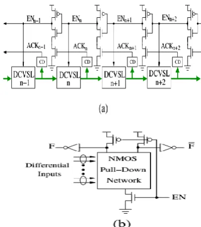
stage is implemented using dynamic differential cascode voltage switch logic (DCVSL) [12] as illustrated in Fig. 1(b). The data validity information in support of self-timed operation is embedded into the dual-rail signaling of the DCVSL logic: When the dual-rail output F and F are both 0, it represents an invalid datum; when one of F and F switches to 1 during evaluation (EN=1), it represents a valid datum (1 or 0). The completion detector (CD) at each stage, as shown in Fig. 1(a), generates 1 when it detects valid data, otherwise generates 0.
The basic idea of zero-delay-overhead self-timed pipeline is to make each DCVSL stage keep ready-to-evaluate status so that it can start the evaluation as soon as tokens arrive, hence tokens can propagate through the pipeline without being blocked (or delayed) by handshake. According to the pipeline as shown in Fig. 1(a), the operation of zero-delay-overhead self-timed pipeline can be described as follows: The pipeline is initialized in such a way that each stage generates invalid output data (i.e., each ACKi is 0) and is ready to evaluate (i.e., each ENi is 1). Once valid data enter the pipeline and reach stage n, stage n starts the evaluation; after finishing the evaluation, it outputs valid data to its successor (i.e., stage n + 1) that will subsequently start the evaluation. The output valid data of stage n will invoke ACKn switch from 0 to 1. As both EN n and ACK n are 1, according to Fig. 1(a), ENn−1 will switch from 1 to 0, leading to the precharge of stage n − 1. In the same manner, after the stage n + 1 finishes the evaluation and generates valid data, stage n + 2 will start to evaluate and stage n will be precharged (i.e., ENn switches from 1 to 0). Clearly, ENn=0 will make ENn−1 switch back to 1 so that stage n − 1 becomes ready to receive and evaluate new valid data. In this way, valid data can propagate through the pipeline data path. The name zero-delay overhead comes from the fact that the forward propagation latency exactly equals the function block latency without any extra delay incurred by self-timed handshake as in many other self-timed pipeline design styles.
Fig. 1: (a) Zero-delay-overhead self-timed pipeline structure, and (b) DCVSL structure.
Such high speed performance comes at the cost of degraded robustness, i.e., to guarantee the correct functionality, the precharge of a stage must be faster than the evaluation of its successor. This assumption is practically reasonable and can be easily satisfied in the real implementations. Finally, we note that the dual-rail dynamic logic DCVSL is self-consistent with such zero-delay-overhead self-timed handshake and can provide a 2x speed performance advantage compared with conventional static CMOS logic. As the cost, dynamic circuits generally suffer from higher power dissipation and less noise immunity.
III. DESIGN OF PASTA
In this section, the architecture and theory behind PASTA is presented. The adder first accepts two input operands to perform half additions for each bit. Subsequently, it iterates using earlier generated carry and sums to perform half-additions repeatedly until all carry bits are consumed and settled at zero level.
A. Architecture of PASTA
It will initially select the actual operands during SEL=0and will switch to feedback/carry paths for subsequent iterations using SEL=1. The feedback path from the HAs enables the multiple iterations to continue until the completion when all carry signals will assume zero values
Fig. 2: General block diagram of PASTA
B. State Diagrams
In Fig. 3, two state diagrams are drawn for the initial phase and the iterative phase of the proposed architecture. Each state is represented by (Ci+1Si) pairwhereCi+1, Si represent carry out and sum values, respectively, from the ith bit adder block. During the initial phase, the circuit merely works as a combinational HA operating in fundamental mode. It is apparent that due to the use of HAs instead of FAs, state (11) cannot appear.
During the iterative phase (SEL=1), the feedback path through multiplexer block is activated. The carry transitions (Ci) are allowed as many times as needed to complete the recursion. From the definition of fundamental mode circuits, the present design cannot be considered as a fundamental mode circuit as the input–outputs will go through several transitions before producing the final output. It is not a Muller circuit working outside the fundamental mode either as internally; several transitions will take place, as shown in the state diagram. This is analogous to cyclic sequential circuits where gate delays are utilized to separate individual states.
Fig. 3: State diagrams for PASTA. (a) Initial phase. (b) Iterative phase
C. Recursive Formula for Binary Addition
Let S ji andC j i+1 denote the sum and carry, respectively, for ith bit at the jth iteration. The initial condition (j =0) for addition is formulated as follows
The jth iteration for the recursive addition is formulated by
The recursion is terminated at kth iteration when the following condition is met:
Now, the correctness of the recursive formulation is inductively proved as follows.
Theorem 1: The recursive formulation of (1)–(4) will produce correct sum for any number of bits and will terminate within a finite time.
Proof: We prove the correctness of the algorithm by induction on the required number of iterations for completing the addition (meeting the terminating condition).
Basis: Consider the operand choices for which no carry propagation is required, i.e., C0
correct result by a single-bit computation time and terminate instantly as (4) is met.
Induction: Assume that Ck
i+1≠0 for something bit at kth iteration. Let l be such a bit for which Ck
l+1 =1. We show that it will be successfully transmitted to next higher bit in the (k+1)th iteration. As shown in the state diagram, the kth iteration of lth bit state (Ck
l+1,Skl) and (l +1)th bit state Ckl+2,Skl+1) could be in any of (0,0), (0,1),or(1,0) states. As Ck
l+1 =1, it implies that Sk
l =0. hence, from (3),Ck+1l+1 =0 for any input condition between 0to l bits.
We now consider the (l +1)th bit state (Ck
l+2,Skl+1) for kth iteration. It could also be in any of (0,0), (0,1),or(1,0) states. In(k+1)th iteration, the(0,0)and(1,0)states from the kth iteration will correctly produce output of(0,1) following (2) and (3). For(0,1) state, the carry successfully propagates through this bit level following (3).
Thus, all the single-bit adders will successfully kill or propagate the carries until all carries are zero fulfilling the terminating condition. The mathematical form presented above is valid under the condition that the iterations progress synchronously for all bit levels and the required input and outputs for a specific iteration will also be in synchrony with the progress of one iteration. In the next section, we present an implementation of the proposed architecture which is subsequently verified using simulations.
IV. IMPLEMENTATION
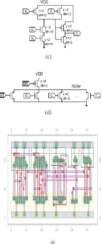
A CMOS implementation for the recursive circuit is shown in Fig. 3. For multiplexers and AND gates we have used TSMC library implementations while for the XOR gate we have used the faster ten transistor implementation based on transmission gate XOR to match the delay with AND gates [4]. The completion detection following (4) is negated to obtain an active high completion signal (TERM). This requires a large fan-in n-input NORgate. Therefore, an alternative more practical pseudo-nMOS ratioed design is used. The resulting design is shown in Fig. 3(d).
Fig. 3: CMOS implementation of PASTA. (a) Single-bit sum module. (b) 2×1 MUX for the 1 bit adder. (c) Single-bit carry module. (d) Completion
signal detection circuit.
V. SIMULATION RESULTS
PASTA:
Synthesis Results:
RTL Schematic:
Technology Schematic:
Design Summary:
VI. CONCLUSION
delay-overhead self-timed pipeline in this context and realize run-time pipeline depth control. Simulations under variable data rate scenarios demonstrate a significant performance gain. It is our hope that this work will motivate the real life adaptive signal processing system designers to re-think their design from a self-timed perspective integrally at the algorithm, architecture, and circuit levels for potential system performance improvement.
REFERENCES
[1] B. Widrow and S. D. Stearns, “Adaptive Signal Processing,” Prentice Hall, 1985.
[2] S. Haykin, “Adaptive filter theory,” Prentice Hall, 1996.
[3] N. R. Shanbhag and K. K. Parhi, “Pipelined Adaptive Digital Filters,” Kluwer, 1994.
[4] T. Williams, “Self-Timed Pipelines (Chapter 9 in Design of HighPerformance Microprocessor Circuits edited by A. Chandrakasan et al.),” John Wiley & Sons, 2000.
[5] J. Sparso and S. Furber, “Principles of Asynchronous Circuit Design: A Systems Perspective,” Kluwer Academic Publishers, 2002.
[6] M. Singh, J. A. Tierno, A. Rylyakov, S. Rylov, and S. M. Nowick, “An adaptively-pipelined mixed synchronous-asynchronous digital FIR filter chip operating at 1.3 gigahertz,” in Proc. Eighth International Symposium on Asynchronous Circuits and Systems, April 2002, pp. 84– 95.
[7] A. Efthymiou and J. D. Garside, “Adaptive pipeline depth control for processor power-management,” in Proc. IEEE International Conference on Computer Design: VLSI in Computers and Processors, Sept. 2002, pp. 454–457.
[8] T. E. Williams and M. A. Horowitz, “A zero-overhead self-timed 160-ns 54-b CMOS divider,” IEEE Journal of Solid-State Circuits, vol. 26, no. 11, pp. 1651–1661, Nov. 1991.
[9] T. D. Howell, W. L. Abbott, and K. D. Fisher, “Advanced read channels for magnetic disk drives,”
IEEE Transactions on Magnetics, vol. 30, no. 6, pp. 3807–3812, Nov. 1994.
[10] C. Ruemmler and J. Wilkes, “An introduction to disk drive modeling,” Computer, vol. 27, no. 3, pp. 17–28, March 1994.