Exploiting sensor mobility and covariance sparsity for distributed tracking of multiple sparse targets

R E S E A R C H

Open Access

Exploiting sensor mobility and covariance

sparsity for distributed tracking of multiple

sparse targets

Guohua Ren

, Vasileios Maroulas

and Ioannis D. Schizas

Abstract

The problem of distributed tracking of multiple targets is tackled by exploiting sensor mobility and the presence of sparsity in the sensor data covariance matrix. Sparse matrix decomposition relying on norm-one/two regularization is integrated with a kinematic framework to identify informative sensors, associate them with the targets, and enable them to follow closely the moving targets. Coordinate descent techniques are employed to determine in a distributed way the target-informative sensors, while the modified barrier method is employed to minimize proper error

covariance matrices acquired by extended Kalman filtering. Different from existing approaches which force all sensors to move, here, local updating recursive rules are obtained only for the target-informative sensors that can update their location and follow closely the corresponding targets while staying connected. Simulations advocate that the proposed scheme outperforms alternative tracking schemes while accurately tracks multiple targets by imposing mobility only on the target-informative sensors.

Keywords: Mobile sensor networks, Distributed processing, Sparse decomposition, Multi-target tracking

1 Introduction

In recent years, potential applications of sensor networks (SN) have expanded due to the low cost of the sensing units, their ability to cover large areas, and the robustness distributed processing offers. One characteristic exploited more and more in sensor networks is sensor mobility and the design of kinematic rules that control sensor move-ment. Sensor mobility adds extra flexibility to a sensor network making it capable of covering larger areas, as well as being more energy efficient and robust [1]. Mobile sensors have been extensively utilized in target tracking applications to enable sensors to closely follow the moving target(s) and provide accurate target location estimates [2–4]. The aforementioned approaches require all the sen-sors to keep active [2–4], which may lead to excessive resource consumption despite the targets’ locality and the fact that in practice a small portion of sensors may pos-sess useful information about the present targets. The aim here is to design an adaptive scheme that exploits mobility

*Correspondence: [email protected]

1Department of Electrical Engineering, University of Texas at Arlington, Arlington, TX, USA

Full list of author information is available at the end of the article

and covariance sparsity to associate targets with sensors and then properly determine kinematic strategies only for the informative sensors which will closely follow the field targets.

In the absence of sensor mobility, there has been a plethora of approaches for tracking multiple targets while associating targets with sensor measurements. Existing works [5–8] associate measurements acquired at static sensors with targets across time and rely heavily on prob-ability models. A distributed Kalman filtering scheme is proposed in [9] relying on information diffusion strate-gies. In [9], only neighboring sensors collaborate, though all sensors in the network are utilized to track a sin-gle source while sensors have fixed locations. A different approach is followed in [10], where consensus-averaging is employed across the whole sensor network and all the sensors are forced to be active irrespective of the quality of their measurements. In [11], a related single-target distributed tracking approach is proposed, in which extended Kalman filtering is employed for tracking. A probability model is assumed to determine informative sensors which may lead to instability due to its depen-dence on the tracking estimates. Different in this paper,

distributed tracking of multiple targets will be considered, while sensor mobility will be exploited and combined with a sensor-to-target association scheme for selecting target-informative sensors without the need of relying on model parameters and state estimators that maybe inaccurate and result divergence. It should be pointed out that the distributed characterization here is referring to the fact that (i) only neighboring sensors need to communicate with each other and collaborate for multi-target tracking, while (ii) processing will take place in a few head sen-sors and will not involve all sensen-sors in the network but only those sensors that bear information about the moving targets.

Single-target tracking using mobile sensor networks has been studied for a variety of different scenarios [12–14]. Most of these approaches control the movement of all sensors by minimizing the estimation error covariance, [4, 13], while the approach in [12] manages sensor mobil-ity based on a Bayesian estimation model and restricting sensors to move only on a grid of locations. A path plan-ning strategy for a setting involving a fixed-location target and a single moving sensor is designed in [15] by maxi-mizing the determinant of the Fisher information matrix corresponding to the configuration. In [16], an approach is proposed for controlling the trajectories of multiple UAVs by minimizing the localization uncertainty for a fixed-location target setting where the target is emitting a radio signal. The work in [17] rigorously presents how sensor mobility can increase spatial resolution when tracking a target with mobile sensors.

When tracking multiple targets with mobile sensors, the approach in [3] proposed an active sensing model, whereas the target-sensor association is based on a near-est neighbor rule which heavily relies on the accuracy of the state estimator while a central processing center is required. The scheme in [18] tackled the problem of mov-ing sensors usmov-ing a flock control law where all sensors are utilized, while the targets are some of the moving sensors whose position is known. The approach in [19] is utilizing clustering and neural networks to move sensors under the assumption that target locations are available. The scheme in [20] designs a Kalman filtering approach with gradient descent-based kinematic rules under the assumption that it is known which targets every sensor observes bypassing in that way the essential sensor-to-target association step. These schemes involve movement of all sensors at every time instant leading to resource-demanding algorithms that do not exploit spatial locality of the field targets.

Measurements corresponding to sensors which are close to the same target tend to be statistically correlated. Given that targets are spatially localized and affect small portions of the sensor network, an approximately sparse sensor data covariance matrix is emerging. Sparsity (pres-ence of a many zero entries in a vector or matrix) has

been exploited in a wide range of applications includ-ing sparse regression and statistical inference, e.g., see [21, 22]. The problem of associating targets to sensors, as well as determining the sensors with target-informative measurements, is formulated here as the task of decom-posing a matrix into sparse factors. The sparse matrix factorization techniques in [23, 24] are integrated here with proper sensor kinematic strategies and tracking tech-niques to exploit sensor mobility. Note that in [23, 24], a stationary (immobile) sensor network is considered where sensors have fixed locations. Tracking in [23, 24] is performed by immobile sensors, whereas here track-ing is generalized to a mobile network with the more challenging task of designing and integrating with multi-target tracking, sensor kinematic strategies that improve tracking accuracy while preserving local sensor network connectivity. Norm-one and norm-two regularization mechanisms are employed to formulate a pertinent min-imization framework that recovers sparse covariance fac-tors, while estimates the number of targets on the field. Coordinate descent techniques [25, 26] are employed to derive local updating recursions that allow sensors to associate with targets.

Different from the aforementioned tracking schemes using sensor mobility, here, only the target-informative sensors will be enabled to move at every time instant and track closely the moving targets. Thus, only target-affected portions of the sensor network will be used for tracking the moving targets, potentially resulting better resource consumption and prolongation of the network lifetime. Kinematic rules will be designed by minimizing proper error covariance matrices obtained by extended Kalman filtering recursions [27] used to track each of the targets. The minimization will be performed under con-nectivity constraints that ensure the moving sensors stay connected and are able to communicate. The modified barrier method ([26], pg. 423) is employed to solve a per-tinent constrained minimization problem and obtain dis-tributed kinematic rules that the mobile sensors can apply locally without the need of a central controller. In contrast to existing approaches, the novel framework identifies and controls the movementonlyof target-informative sensors allowing for accurate tracking.

takes local sensor network connectivity into account to ensure that the tracking process carries out continuously; and (v) different from [15, 16] that consider fixed-location target(s), here, kinematic strategies are developed for trackingmultiple movingtargets. The proposed approach here achieves this task only by using the sensor data and sparsity-imposing mechanisms.

The paper is structured as follows. The problem formulation and setting are given in Section 2. The sensor-to-target association scheme which provides the target-informative sensors is delineated in Section 3.1 and is combined with extended Kalman filtering techniques in Section 3.2. Novel kinematic rules are developed in Section 3.3 after minimizing a pertinent error covariance matrix under connectivity constraints and employing the modified barrier method to derive local kinematic rules that enable the target-informative sensors to update their location and follow closely to moving targets. The pro-posed algorithmic framework is detailed in Section 4.1, while the communication and computational costs are discussed in Section 4.2. Extensive numerical tests are car-ried out in Section 5 that corroborate the advantages of the novel method over existing alternatives.

2 Problem setting

An ad hoc sensor network conformed bypmobile sen-sors is considered here. The sensen-sors monitor a field where an unknown and possibly time-varying number of moving targets is present. Each sensor communicates only with its neighboring sensors which are within its communica-tion range and are able to exchange informacommunica-tion with a single-hop of communication. The single-hop neighbor-hood of sensorjis denoted asNj(t), wheretdenotes the time index.

In general, all targets are assumed to be moving in aK-dimensional space. Then, every target, say the ρth, is characterized by a 2K × 1 state vector which con-tains both its position coordinates and velocity informa-tion for each coordinate. The posiinforma-tion coordinates for the ρth target at time t are stacked in vector pρ(t) =

p_ρ,x1(t),. . .,pρ,xK(t) T

, while the velocity per coordinate is in vectorvρ(t) = vρ,x1(t),. . .,vρ,xK(t)

T

. So at timet, the state vector can be written assρ(t)=pT_ρ(t),vT_ρ(t)T, while it evolves according to a near constant veloc-ity model [28]. Specifically, the ρth target’s state vec-tor evolves according to the following constant velocity model, see e.g., [28]:

sρ(t+1)=Fsρ(t)+uρ(t), (1)

whereFis the 2K×2Kstate transition matrix anduρ(t) the zero-mean Gaussian state noise with variance u. MatricesFanduare given as follows:

F=

⎡ ⎢ ⎢ ⎢ ⎢ ⎢ ⎣

1 0 . . . T . . . 0 ..

. ... ... ... ... ... 0 1 0 0 . . . T 0 0 1 . . . 1 0 0 0 0 . . . 0 1

⎤ ⎥ ⎥ ⎥ ⎥ ⎥ ⎦

,

u=σ2 u

(T)3/3·IK (T)2/2·IK (T)2_/2·I

K T·IK

,

(2)

whereσ_u2is the noise variance andIK denotes the iden-tity matrix of sizeK×K, whileTdenotes the sampling period.

Sensorjsenses the moving targets, by acquiring at time ta scalar measurement depending on the target location according to the following nonlinear model:

xj(t)=R_ρ= 1aρ(t)d

−2

j,ρ(t)+wj(t), j=1,. . .,p, (3) whereaρ(t)denotes the intensity of a signal emitted from theρth target anddj,ρ(t)= pj(t)−pρ(t)is the distance between sensorjand the ρth target at timet. The total number of targets which move in the field through the lifespan of the SN is indicated asR, whilewj(t)denotes the white sensing noise with varianceσ2

wand zero-mean. The following assumptions are introduced in the considered setting:

• A1: In the measurement model in (3), it is assumed

that the targets act as transmitters and each sensor will receive one reflection of the signal emitted from the targets. Signals emitted from the targets

propagate via free space, explaining thed−_j,ρ2(t)

attenuation coefficients, and are superimposed as shown in (3), see e.g., [29].

• A2: The signal amplitudesaρ(t)are considered to be uncorrelated across the different targets.

• A3: Among the summandsaρ(t)d−j,ρ2(t)in (3), only

one has a large amplitude when sensorj is close to theρth target, whereas others are negligible due to the square-law attenuationd−_j,ρ2(t)caused by the free space propagation.

Note that assumption A3 corresponds to a setting where at most, one target is present within the sensing range of a sensor. Note that this is a more relaxed version of the common assumption that one sensor just contains the measurement of a specific target [6–8]. The signal ampli-tudesaρ(t)will be nonzero for the interval in which the corresponding target is active and moving while is kept at zero when the target is inactive and disappears.

[16]. The deployed sensors are listening for these signals to track the moving entities. The targets could correspond to independent entities; thus, it is expected that the infor-mation bits they transmit are uncorrelated, giving rise to uncorrelated transmission signals [30]. Thus, the commu-nication radio signals that the targets may be emitting are utilized to perform tracking and move the sensors appro-priately. Applications include localization and tracking of mobile users in wireless networks, as well as tracking of vehicles in tactical environments [16].

Stacking all the sensor measurements in (3) on ap×1 vector, it follows:

xt=Dtat+wt, whereat:=[a1(t)a2(t) . . .aR(t)]T, (4)

whereDtis ap×Rmatrix with entriesDt(j,ρ)=d_j−,ρ2(t) with j = 1,. . .,pand ρ = 1,. . .,R. The noisewt has covariancew = σ2

wIp. Given that the entries ofat are uncorrelated, it follows readily that the data covariance matrix is

x,t=DtaDTt +σw2Ip= ¯DtD¯Tt +σw2Ip, (5)

where a is the diagonal covariance matrix of at, while ¯

Dt:=Dta1/2. Among theRentries inat, there will ber(t) nonzero entries corresponding to the active targets mov-ing at the sensed field att. In the setting here, once a target becomes inactive (i.e.,aρ(t) = 0), it remains inactive for the rest of time.

The goal is to enable the mobile sensors to track an unknown number of targets present in the monitored field. Novel target association and sensor mobility strate-gies will be combined with tracking techniques to enable sensors to accurately track the different target trajecto-ries. Proper kinematic strategies will be developed to allow only a small percentage of target-informative sensors to move, different from existing approaches [12, 14] where all sensors are moving at every time instant that may be more resource demanding. Judiciously selecting and moving sensors will enable target tracking even when the targets move outside the area originally monitored by the sensors.

3 Distributed association, tracking, and sensor kinematic strategies

3.1 Target-informative sensor selection

Due to the presence of multiple target in the moni-tored field, the first goal is to determine sets of sensors, namely Sρ,t, that acquire information bearing measure-ments about theρth target. From the observation model in (4), note that the strong-amplitude entries of the ρ column in Dt, namely {Dt,:ρ}Rρ=1, can reveal the sen-sors within subsetSρ,t. Specifically, recall thatDt(j,ρ) =

d_j−_,ρ2(t); thus, when sensorjand targetρare close in dis-tance then the corresponding entry is expected to have large amplitude, while the further away they get from each other the closer to zero the corresponding entry gets. The matrixDtcan be assumed approximately sparse. Thus, the strong-amplitude entries (away from zero) inDt,:ρcan be used to determine the informative sensor members ofSρ,t at time instantt. Thus, determiningSρ,tboils down to the problem of recovering the support of the columns ofDt.

To recover the sparse matrixD¯tin (4), the data covari-ance matrix will be decomposed into sparse factors. Due to the fact that the targets and sensors may be moving while the number of targets is changing, the sparse sensor data covariancex,tis also time-varying. In practice, the ensemble covariance is not available and needs to be esti-mated. To this end, exponential weighing is employed to estimate the time-varying covariance entries. The notion of exponential weighing in recursive least-squares used in processing non-stationary signals, see e.g., ([31], Ch. 9), is estimating the time-varying covariance matrix here as follows:

ˆ x,t=

1−ω 1−ωt+1

t

τ=0ωt−τ(xτ− ¯xt)(xτ − ¯xt)T, (6) whereω∈(0, 1)denotes a forgetting factor and

¯ xt=

1−ω 1−ωt+1

t

τ=0ωt−τxτ, (7) corresponds to a real-time estimate for the ensemble mean at time instantt. Note thatωin Eqs. (6) and (7) is used in a way that puts more emphasis to the recent data while it gradually forgets the past data, which is exactly what an up-to-date estimator needs to do for the time-varying setting considered here. The scaling(1−ω)(1− ωt+1₎−1_{in (6) and (7) is to ensure that the two estimates}

ˆ

x,tandx¯tfor the ensemble quantitiesx,tandE[xt] will be unbiased.

To account for the nearly sparse structure of D¯t, the unknown number of targets and single-hop connectivity of the sensor nodes the following formulation relying on norm-one/norm-two regularization is utilized:

ˆ

Mt,{ ˆσj}mj=1

:=arg min Mt,{σj}mj=1

Eˆx,t−MtMTt

−diag

σ2

1,t,. . .,σp2,t

2 F

+ L

=1

λMt,:1+φMt,:2

,

(8)

active sensed targetsr(t)(L ≥r(t)) andMt ∈ Rp×L con-tainsLcolumns that estimate the sparse columns ofD¯t. Mt,:denotes theth column ofMt. The formulation was first proposed in [23, 24] to perform target-sensor associ-ation in a network of stassoci-ationary sensors that do not have moving capabilities. Here, this formulation will be uti-lized to determine the different sets of informative sensors observing different targets before being integrated with kinematic control rules.

The Hadamand operator along with the adjacency matrix E in (8) allows only the single-hop covariance entries to be used since they can be calculated by direct communication of the corresponding neighboring sen-sors. The first term in (8) accounts for the structure in (5). Sparsity is induced in the columns of Mt using the norm-one term in (8), (see e.g., [22]), whileλ denotes the nonnegative sparsity-controlling coefficient used to adjust the number of zeros in Mˆt,:. The coefficient φ ≥ 0 in the last term of (8) promotes group sparsity among rows, [32], thus is introduced to adjust the num-ber of nonzero columns of Mˆt needed to approximate

ˆ

x,t. This is done to zero-out unnecessary columns inMˆ when the number of active targets in the field is smaller than R. The number of nonzero columns in Mt indi-rectly estimates the number of targets at time instant t, namelyˆr(t).

The cost in (8) is minimized by an iterative minimiza-tion scheme based on coordinate descent [25, 26], where sensor j is responsible for updating the jth row of Mt, namelyMt,j:. Specifically, the cost is minimized wrt one entry of Mt or diag(σ12,. . .,σp2), while keeping the rest fixed to their most up-to-date values. Sensorjupdates the entries{Mt(j,)}L₌₁and varianceσ_j2_,t. During one coordi-nate cycle, all the entries ofMtand diag(σ_1,2_t,. . .,σp2,t)will be updated.

The updates for entriesMˆk_t(j,)will be formed by differ-entiating (8) wrtMt(j,)and setting the derivative equal to zero, while fixing the rest of the entries ofMtandσj,tto their most recent updates inMˆk_t−1and{σ_j2_,t,k−1}evaluated at cyclek−1. It turns out (details in [23, 24]) that during coordinate cyclek, the updateMˆk_t(j,)can be obtained as the value that gets the minimum possible cost in (8) (while fixing the rest of the variables) among the candidate val-ues: (i)z=0; (ii) the real positive roots of the third-degree polynomial

z3+ ⎡

⎣

i∈Nj

[Mˆk_t−1(i,)]2−ψ_tk_,(j,j,)+ φ 2

⎤

⎦ (9)

z− ⎡

⎣

i∈Nj ψk

t,(j,μ,)Mˆkt−1(i,) ⎤ ⎦₊ λ

4 =0

and (iii) the real negative roots of the third-degree polynomial

z3+ ⎡

⎣

i∈Nj

[Mˆk_t−1(μ,)]2−ψ_tk_,(j,j,)+ φ 2

⎤

⎦ (10)

z− ⎡

⎣

i∈Nj ψk

t,(j,i,)Mˆkt−1(i,) ⎤ ⎦₋λ

4 =0

where

ψk

t,(j,i,):= ˆx,t(j,i)−δj,iσˆj2,t,k−1 (11) −

L

_=1,= ˆ

Mk_t−1j,Mˆk_t−1i,, whileδj,idenotes the Kronecker delta function, i.e.,δj,i=1 ifj=i, andδj,i=0 ifj=i. The roots of the two aforemen-tioned polynomials can be calculated using companion matrices, see e.g., [33].

Furthermore, during cyclekat time instantt, the noise variance estimates across sensors can be updated as

ˆ σ2

j,t,k = ˆx,t(j,j)− ˆMkt,j:

ˆ Mk_t,j:

T

, j=1,. . .,p. (12)

Sensorjneeds to communicate only with its single-hop neighbors inNj, in order to evaluate the coefficients of the polynomials in (9) and (10) and to update the noise vari-ance estimates in (12). It can be shown that ask → ∞, the updatesMˆk_t−1converge at least to a stationary point of (8). Further, the sparsity-controlling coefficients{λ}L₌1 can be set using the strategy proposed in ([23], Sec. V.A). Once the sparse columns{ ˆMt,:}are estimated, their sup-port (the indices of relatively strong-amplitude entries) is used to determine which sensors sense a specific target at timet.

3.2 Tracking via extended Kalman filtering

The target-informative sensor subsets Sρ,t for = 1,. . .,r(t)ˆ , whereˆr(t) corresponds to an estimate of the number of targets at time instant t obtained from the number of nonzero columns ofMˆt := ˆMKt¯, after apply-ing K¯ coordinate cycles. Extended Kalman filtering is employed to process the nonlinear observations and track each target’s location using the observations of the cor-responding set Sρ,t. For simplicity in exposition, the specifics of extended Kalman filtering (EKF) will be delin-eated here forK = 2 dimensions, but it can be readily generalized to more dimensions. The target state estima-tor and corresponding error covariance matrix, obtained by the extended Kalman filter using the observations in

the following updating recursions for the state estimator and covariance at time instantt

ˆ

sρ(t+1|t)=Fˆsρ(t|t), Mρˆ (t+1|t)=FMρˆ (t|t)FT+u. (13)

The measurements of the sensors within set Sρ,t will then be used to carry out the correction step of the extended Kalman filter which involves the following update recursions:

ˆ

sρ(t+1|t+1)= ˆsρ(t+1|t)+K(t+1) (14) ·xt+1−aρ(t)DˆS_ρ,t

Mρ(t+1|t+1)=Mρ(t+1|t)+DT∇,ρ(t+1|t) ·σ2

wI|S_ρ,t|·D∇,ρ(t+1|t), (15) for=1,. . .,rˆ(t), while the matrixKρ(t+1)corresponds to the Kalman gain given as

Kρ(t+1)=Mρ(t+1|t+1)·DT∇,ρ(t+1|t)·σ 2 wI|S_ρ,t|,

(16)

whereDˆS_ρ,tis a|Sρ,t| ×1 vector whose entries are given by||pj(t)− ˆpρ(t+1|t)||−2

j∈S_ρ,t, in whichpˆρ(t+1|t)

is theρth target position extracted from the state predic-tionsˆρ(t+1|t). Further,D∇,ρ(t+1|t)is the|Sρ,t| ×4 matrix whose rows constitute of gradient∇Dt(j,ρ)with respect to the state vectorsρand evaluated atˆsρ(t+1|t) forj∈Sρ,t, i.e.,

∇sρDt(j,ρ)s_ρ=ˆs_ρ(t+1|t)

=2·

pj,x(t)− ˆpρ,x(t+1|t),pj,y(t)− ˆpρ,y(t+1|t), 0, 0T

(pj,x(t)− ˆpρ,x(t+1|t))2+(pj,y(t)− ˆpρ,y(t+1|t))2

2.

(17)

Within each informative subset of sensorsSρ,t, the sen-sor closest in distance to the predicted position of theρth target, namelyˆsρ(t+1|t), is set as a the subset head sen-sor that will gather the measurements of all other sensen-sors inSρ,tand perform the EKF tracking recursions.

3.3 Sensor kinematics

The focus in this section is to derive kinematic rules for the target-informative sensors, which are selected accord-ing to the scheme in Section 3.1, such that they follow closely the moving targets and give accurate position esti-mates. The benefit from having a few sensors moving is that targets can be tracked even when they move away from the original field monitored by the sensors. Having sensors following closely, the moving targets can provide more reliable measurements about the targets than just using static sensors. Note that only informative sensors

close to the targets will be responsible for carrying out the tracking procedure leading to resource savings. Toward this end, the informative sensors in each subsetSρ will be placed/move in locations that minimize the trace of the error covariance associated with the estimatorsˆρ(t|t). This will ensure that the informative sensors associated with each target move to a location that will provide mea-surements that result good tracking accuracy. The idea of minimizing a scalar function of the predicted error covari-ance was also applied in moving all sensors in a network for trackinga singletarget [2, 3, 12]. Here kinematic strate-gies are derived in the presence of multiple targets, while a judiciously selected small portion of target-informative sensors will be moving instead of all sensors moving.

Among the two terms in the covariance matrix in Eq. (15), only the second term is affected by the sensors’ location. The latter term, after using (17), can be written as:

j∈Sρ,t

4

(pj,x(t+1)− ˆpρ,x(t+1|t))2+(pj,y(t+1)− ˆpρ,y(t+1|t))2 3.

(18)

Clearly, (18) depends on the position of the sensors asso-ciated with targetρ, namely the sensors in subsetSρ,t, at time instantt. Lettingpj(t+1):=[pj,x(t+1) pj,y(t+1)]T notice that the trace cost in (18) is separable with respect to the position of each sensorjwithin subsetSρ,t. Thus, the position of sensor j ∈ Sρ,t at time instantt+ 1 is determined by minimizing the corresponding summand in (18), i.e., the updated location for sensorsj∈Sρ,tcan be found as

pj(t+1)=arg minpj,x,pj,y

4

pj,x− ˆpρ,x(t+1|t) 2₊

pj,y− ˆpρ,y(t+1|t) 23

s. topj,x− ˆpρ,x(t+1|t)2+pj,y− ˆpρ,y(t+1|t)2<R2

(19)

Note that the inequality constraint in (19) ensures that the new location of the moving sensors j ∈ Sρ will be within distanceRjfrom the latest target location estimate

ˆ

pρ(t+1|t). This inequality further ensures that all sensors inS_ρ will move to new locations which are “close” to the target. After applying the triangle inequality for the new locations of two sensorsjandjwithinSρ and using the constraint in (19), it turns out that the new location should satisfy

pj(t+1)−pj(t+1)2≤ √

2R, (20)

sensors and perform clustering. Details of the algorithm are given in Section 4.1. Note that existing approaches do not entail mechanisms as the one introduced here to ensure that sensors will be connected.

Next, the modified barrier method (MBM) is utilized ([26], pg. 423) to allow every sensor j ∈ Sρ to solve (19) and determine its next location. To this end, let f(pj) denote the cost in (19) and g(pj) denote the left hand side function of the inequality constraint in (19). MBM involves an iterative application of the following unconstrained minimization problem (where κ denotes the iteration index within time instantt+1):

pκ_j(t+1)∈arg min pj,x,pj,y

f(pj)+ μ

κ

cκ φ

cκ·g(pj),

(21)

where the Lagrange multiplier-like scalarμκis updated as

μκ+1_=μκ _{· ∇φc}κ_·g(pκ j(t+1))

, (22)

while the barrier functionφ[τ] is chosen as a logarith-mic function having the form

φ(τ)= −ln(1−τ) (23)

andcκis a penalty parameter associated with the inequal-ity constraint in (19) that is updated according to the recursion

cκ = γ κ

μκ (24)

where{γk} is a positive monotonically increasing scalar sequence [26].

For the logarithmic barrier function in (23) the updat-ing recursion of the multipliers in (22) takes the followupdat-ing form

μk+1₌ μκ

1−cκg(pκ_j(t+1)). (25)

Further, letting F(pj) := f(pj)+ μ_cκκφcκ ·g(pj), the coordinates of the new sensor location pj(t + 1) are updated during iteration κ according to the following gradient descent recursions

pκ_j,x+1(t+1)=p_jκ_,x(t+1)−·dF(pj) dpj,x

pj,x=pκj,x(t+1)

(26)

pκ_j,y+1(t+1)=p_jκ_,y(t+1)−· dF(pj) dpj,y

pj,y=pκj,y(t+1)

(27)

whereis the step size for the gradient descent method, while the derivatives in (26) are given as

dF(pj) dpj,x

pj,x=pκj,x(t+1)

= 24·

−pκ_j,x(t+1)+ ˆp_ρ,x(t+1|t)

pκ_j,x(t+1)− ˆpρ,x(t+1|t)

2

+pκ_j,y− ˆpρ,y(t+1|t)

24

+ μκ

1−cκg(pκ_j(t+1))·2·(p

κ

j,x(t+1)− ˆpρ,x(t+1|t)),

dF(pj) dpj,y

pj,y=pκj,y(t+1)

= 24·

−pκ_j,y(t+1)+ ˆp_ρ,y(t+1|t)

pκ_j,x(t+1)− ˆp_ρ,x(t+1|t)

2

+pκ_j,y(t+1)− ˆp_ρ,y(t+1|t)

24

+ μκ

1−cκgpκ_j(t+1)·

2·pκ_j,y(t+1)− ˆp_ρ,y(t+1|t)

.

(28)

During time instant t + 1, each sensor j within the subset Sρ,t will keep updating their location until the cost function in (19) is not reduced more than a prede-fined threshold within two consecutive updating steps κ,κ+1. The locationpj(t+1)will be set to the last update

pK_j (t+1)obtained afterKMBM iterations during time instantt+1. The following steps are carried out during the determination of the sensor’s new location:

S1) The head sensor in each subsetSρ,tsends the pre-dicted position estimate of targetρ, namelypˆρ(t+1|t), to all sensors inSρ,t.

S2) Each sensor inj ∈ Sρ,t, determines its new loca-tion using the MBM scheme. Sensors inSρ,tcheck their distances to other neighboring sensors, and if their future location is too close, they adjust their coordinates to avoid collision when moving. Similarly, each moving sen-sor checks the distance between its updated location and the position estimate of targetρ, and if too close, adjust-ments will be made to the sensor’s location such that a minimum distance will be kept from the target. Specifi-cally, if sensorjhas an updated locationpK_j(t+1)which is too close to the already updated location of sensorj, namelypj(t+1), i.e.,pK

j (t+1)−pj(t+1)2≤Rmin,a, whereRmin,ais the smallest distance allowed that two sen-sors can be separated from each other, thenpK_j(t+1)is updated as follows:

pj(t+1)=pj(t+1)+Rmin,a

pK_j(t+1)−pj(t+1) pK_j(t+1)−pj(t+1)2

.

(29)

pK

j (t+1)− ˆpρ(t+1|t)|2 ≤ Rmin,bwhereRmin,bis the smallest distance that a sensor can be placed from a target, then locationpK_j(t+1)is updated as follows:

pj(t+1)= ˆpρ(t+1|t)+Rmin,b

pK_j(t+1)− ˆpρ(t+1|t) pK_j(t+1)− ˆpρ(t+1|t)2

.

(30)

The collision-avoidance position modifications in (30) were proposed in [34] to prevent collision of unmanned aerial vehicles with a stationary target. The position updates in (29) and (30) ensure that the updated locations are at distanceRmin,aandRmin,bfrom another moving sen-sor or moving target, respectively, satisfying the minimum distance required to prevent collision.

The actual movement can be achieved using for example robotic sensors, see e.g., [35, 36]. Each sensor j ∈ Sρ,t updates its locationpj(t+1), in a coordinate fashion while the remaining sensors inSρ,tare kept stationary waiting for their turn to update their location.

4 Algorithmic summary 4.1 Implementation

At the start-up stage, fast sampling is used to acquireQ measurements fast enough that the initial number of tar-gets r(0) can be assumed stationary. By utilizing theQ acquired data, the subsets of target-informative sensors

{Sρ,0} are initialized, where = 1,. . .,ˆr(0) andˆr(0) is the estimated number ofr(0)sensed targets at timet=0 (number of nonzero columns in the sparse matrix Mˆ0). One sensor within each Sρ,0 will be randomly selected as the head sensor, which will collect the measurements xj(0)and their positionspj(0)from all the other sensors j ∈ Sρ,0. Each head sensorCρ,0 averages the positions of the informative sensors in subset Sρ,0 to be the ini-tial estimate of the corresponding target ρ. The latter target location estimate along with the informative mea-surementsxj(0), forj∈ S_ρ,0are utilized to initialize the recursions of the extended Kalman filtering carrying out the target tracking in Section 3.2.

At time instantt, every head sensorCρ,thas available the state estimates for active target ρ, namely ∫ˆρ(t|t), obtained from EKF in Section 3.2. The target’s estimated position pˆρ(t|t) is then used to select a group of “can-didate informative” sensors, which are denoted as J_ρ,t for targetρ at time instantt. This set is formed by hav-ing the head sensor transmit the estimated state∫ˆρ(t|t) to its single-hop neighboring sensors which then trans-mit the same information to their own neighbors. Every sensorjwho receives∫ˆρ(t|t), from a neighboring sensor, subsequently forwards this estimate only to those sensors j ∈ Nj whose present position is within radiusRs from the estimated target location, i.e.,pj(t)− ˆpρ(t|t)2≤Rs. The parameter Rs can be set to be sufficiently large in

order for allρ-target-informative sensors to be incorpo-rated in subsetJρ,t. The sensor subsetJρ,tby construc-tion is connected.

Since not all sensors within the candidate subsets

Jρ,t maybe informative, the scheme in Section 3.1 is employed among the sensors inJρ,tto find out the target-informative sensor subsetSρ,t+1⊆Jρ,tfor all the active targets. Rather than running the target-sensor association scheme in Section 3.1 in the whole sensor network, it is performed independently in the different sensor subsets

Jρ,tassociated with each target.

Once subsetsSρ,t+1are found, the head sensor in each of these subsets is chosen to be the sensor whose distance is the closest to the estimated position of the correspond-ing targetρ, i.e.,

Cρ,t+1=arg min j∈S_ρ,t+1

pj(t)− ˆpρ(t|t)2.

The head sensor Cρ,t+1 gathers the sensor measure-mentsxj(t+1)from the informative sensorsj ∈ Sρ,t+1 to carry out the extended Kalman filtering recursions at time instantt+1 as outlined in Section 3.2. Then, steps S1 and S2 in Section 3.3 are employed to allow all sensors inSρ,t+1to determine and move to their new positions pj(t+1). Note that connectivity of the sensors inS_ρ,t+1 is preserved as explained in Section 3.3. The head sen-sor C_ρ,t+1 broadcasts the latest state estimate sˆρ(t + 1|t+1)to its single-hop neighbors and repeats the pro-cess described earlier to update the candidate informative sensor subsetsJρ,t+1.

It is worth mentioning that the kinematic rules imple-mented in Section 3.3 at each sensor are fully distributed since each sensor requires knowledge only of its location and the estimated target position obtained from the head sensor inSρ,t+1. Connectivity of the candidate informa-tive subsetsJρ,t+1is ensured by construction irrespective of the sensor movement. This way the sensor-to-target association scheme in Section 3.1 can still be applied in

Jρ,t+1and determine the informative sensors.

update the sensor-informative subsets. The novel tracking scheme is summarized as Algorithm 1.

Algorithm 1Multi-target tracking using sensor mobility and informative sensor selection

1: Start-up stage (t = 0)/Reconfiguration (t = 0):Every sensorjcollectsQmeasurements xj(t)and the sensors-targets association scheme in Section 3.1 is applied in the network to determine the subsetsSρ,twith=1,. . .,rˆ(t), andˆr(t)is the estimated number of targets.

2: forτ=t,. . .,do

3: Determine the head sensorCρ,τ in eachSρ,τ for = 1,. . .,ˆr(t).

4: Each head sensor Cρ,τ receives measurements xj(τ) fromj ∈ Sρ,τ to perform tracking for targets ρ =

1,. . .,ˆr(t)via the EKF recursions in Section 3.2. 5: Informative sensors j ∈ Sρ,τ relocate themselves

according to the sensor kinematics introduced in Section 3.3.

6: Each head sensorCρ,τ propagates the state estimates ˆ

sρ(τ)to every sensorjthat can be reached fromCρ,τby a multi-hop path and satisfiespj(τ)− ˆpρ(τ|τ)2<Rs. Then, the candidate informative sets{Jρ,τ+1}ˆr(=t)1 are formed.

7: The sensor selection scheme in Section 3.1 is carried out in each subsetJρ,τ+1to identify the target-informative setsSρ,τ+1.

8: If target configuration has changed then go to step 1, otherwise go to step 2.

9: end for

4.2 Communication and computational expenses The communication cost of the proposed algorithm is studied next. Note that inter-sensor communication takes place during (i) the sensor-to-target association scheme in Section 3.1; (ii) carrying out the EKF tracking steps in Section 3.2; and (iii) when applying the kinematic strategy in Section 3.3 to move the informative sensors. In detail, at time instantt, sensorjhas to receive|Nj|scalar mea-surements from its neighbors, namely{xj(t+1)}j∈Nj, to

updateˆx,t+1(j,j). Furthermore, to implement the asso-ciation scheme in Section 3.1, each sensorjreceives the updates { ˆMk_t+−₁1(j,)}L₌₁ from neighborhood Nj, corre-sponding toL|Nj|scalars in total, to form its local updates { ˆMk_t+1(j,)}L₌₁. Thus, sensorjreceives(L+1)|Nj|scalars in total. Similarly, sensorjhas to transmitxj(t+1)and

{ ˆMk_t+−₁1(j,)}L₌₁, a total ofL+1 scalars to its neighbors, per iterationk.

After the target-informative sensors are determined, each head sensor has to carry out the estimation process about the corresponding target’s states. Thus, the head sensor {Cρ,t} will collect the measurements xj(t) from the sensors within Sρ,t+1. This involves |Sρ,t+1|scalar exchanges. Further, all sensors in the subsetSρ,t+1 will

receive four scalars corresponding to the current state estimate. Once the state estimation process (Section 3.2) is carried out by the head sensors, sensor communica-tion also occurs among the informative sensors when adjusting their new location to avoid collision with closely located sensors (Section 3.3). Specifically, sensorjreceives 2|Nj| scalars from its neighbors, corresponding to their two location coordinates, while it sends out its own loca-tion. It is worth mentioning that the communication complexity for each sensor is linear with respect to its neighborhood size|Nj|, and the upper bound number of present targets L. The latter linear cost advocates that the proposed framework is a communication-affordable distributed approach.

When applying the scheme in Section 3.1 during each coordinate cyclek and time instantt, each sensorjhas to form the coefficients in (10), (9) with a computa-tional complexity of the order O(|Nj|), while determin-ing the roots of the two third-order polynomial in (10), (9) involves determining the eigenvalues of two 3 × 3 companion matrices whose complexity is fixed and non-dependent on any algorithmic parameters. The EKF in Section 3.2 can be carried out at a complexity of the order

O(K2_{+ |S}

ρ|), whereK = 4 here and|Sρ|corresponds to the size of the target-informative subsets. The kine-matic rules implemented at the target-informative sensors in Section 3.3 have a computational complexityO(K).

5 Simulations

0 5 10 15 20 25 30

10−2

10−1

100

101

102

Proposed approach Scheme in [9] Scheme in [2]

Fig. 1Tracking RMSE versus time for a single-target setting

not have an informative sensor selection scheme, which results all sensors to move and participate in the tracking process which may reduce accuracy when noisy sensors are utilized.

Figure 2 depicts the distance (in meters) between two moving sensors and the corresponding moving target dur-ing the 30-s trackdur-ing period. It can be seen that the distance is decreasing with time which further implies that the proposed approach allows the informative sensors to closely follow the target.

Next, the performance of our novel tracking scheme is tested in a setting where the number of targets is chang-ing. Specifically, targetsρ=1, 2 start moving at positions [1.5, 11.5], [ 5, 7] and follow the dynamics in (1), with velocities of [ 0.15, 0.1] and [ 0.4, 0.13] m/s along thex-axis andy-axis, respectively. Targetsρ=1, 2 move in the field for the time interval [1, 30] s and then are not sensed any-more. In the interval [15, 17] s, no targets are present in the field. Then, targetsρ=3, 4 start at positions [6.1, 4.8], [9.0, 4.0] and move according to same state model

0 5 10 15 20 25 30

0 1 2 3 4 5 6

t

Distance (m)

Distance between target and sensor 16 Distance between target and sensor 3

0 2 4 6 8 10 12 14 16 18

Sensor network at t=0

Fig. 3Original sensor network topology (before applying kinematic rules to the sensors)

followed by the first two for the time interval [32, 50] s but with velocities [0.03, 0.35] and [0.25,−0.25] m/s. Again, no targets are present during the interval [50, 52] s. Then, three targetsρ = 5, 6, 7 start moving at positions [15, 1.1], [13, 13.5], and [12, 6], according to (1), for the

time interval [52, 70] s and velocities [−0.1, 0] m/s for target ρ = 5, and [0.12,−0.03] for both ρ = 6, 7 along thex-axis andy-axis, respectively. Figure 3 depicts the original positions of the sensors represented by blue circles.

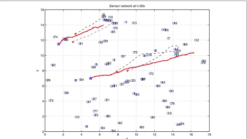
Sensor network at t=30s

x

y

0 2 4 6 8 10 12 14 16 18

Sensor network at t=50s

x

y

Fig. 5Snapshot of the trajectories of targets and moving sensors at time instantt=50 s.Red solid curvescorrespond to the true target trajectories; blue dashed curvesrepresent the estimated track.Blue starsindicate the starting locations of the targets, while thered crossesdenote the initial locations of some moving sensors. Theblack dashed curvesshow the trajectories of some of the moving sensors during the tracking process

Figures 4, 5 and 6 show snapshots of the configura-tion of the targets and the moving sensors at different time instances. Details for the different curves and col-oring on those figures is given in the caption below the figures. From Fig. 4, it is clear that for the first two tar-gets, even though the targets move out of the original

[0, 15]×[0, 15] region, both targets are still tracked well as some of the sensors follow them closely. Note that only informative sensors, on average around 10 % of the total number of sensors, move according to the proposed kine-matic rules in Section 3.3, while the majority of other sensors which are not close to the moving targets are

0 2 4 6 8 10 12 14 16 18

Sensor network at t=70s

x

y

not moving and maintain their original positions. Simi-lar conclusions can be extracted from Figs. 5 and 6, where different sets of targets are moving on the field. It should be emphasized that it is not known that att = 30 and t = 50, the target configuration is changing. As dis-cussed in Section 4, such changes can be determined by having all sensors self-checking the energy level of their measurements, while the head sensors monitor the informative sensor subsets whether they are empty or not.

The tracking RMSE for the above tracking setting is plotted in Fig. 7 in logarithmic scale. The proposed track-ing framework exploittrack-ing sensor mobility is compared with a tracking scheme where sensors are stationary and not moving. In the immobile sensor network, when the targets are moving away from the sensed field, the sensors will acquire less and less reliable measurements leading to the dramatic increase of the tracking RMSE (blue dashed curves). In contrast, the proposed framework here enables sensors to follows closely the targets and achieve a much lower tracking RMSE. So even though the targets move out of the original sensed field, there is always a group of sensors keeping adjacent to it and can be selected again to provide accurate measurements. Note that in Fig. 7, there are three discontinued curves which corresponds to the error of tracking the three different groups of targets that appear and cease to exist in the monitored field at different time periods. This leads to the RMSE discontinuity at time t = 31 s andt = 51 s since there are no targets moving during that time interval and no need for tracking.

Next, a tracking setting is considered with two targets where one of targets splits into two targets at a cer-tain time. Similarly to the previous tracking scenario,

two targets ρ = 1, 2 initialized at positions [1.6, 11.5], [ 5.4, 7] (indicated by the blue stars) start moving according to the dynamics in (1), with velocities of

v1 =[v1,x,v1,y]=[ 0.15, 0.1] m/s and v2 =[v2,x,v2,y]= [ 0.4, 0.13] m/s, respectively. Ast = 30, the second target stops moving while the first one splits into two targets. Targetρ= 3 continues to move according to the dynam-ics of target ρ = 1, while target ρ = 4 moves with velocitiesvx=0.4 m/s andvy= −0.5 m/s along thex-axis andy-axis. The two new targets move for the time interval [ 31, 42] s. The splitting point is indicated by the green star in Fig. 8. Figure 8 shows the trajectories of the targets and some moving sensors; details on the coloring and curve types used can be found in the caption of Fig. 8 . The target trajectories in Fig. 8 are depicted by blue dashed lines for the time interval [ 1, 30] s and by blue crossed lines after t=30 s. When sensors do not move, the violet estimated trajectories indicate that the split of targets cannot be fol-lowed, while targetρ =1 cannot be tracked after a while since is moving away from the immobile sensors. When the kinematic rules in Section 3.3 are employed, infor-mative sensors follow closely the targets as depicted by the black dashed sensor trajectories. Note that the corre-sponding estimated red trajectories accurately follow the multiple targets present in the field. As before, the track-ing RMSE (logarithm) is compared for the cases where sensors cannot move with the case where the approach in Section 3.3 is applied. As Fig. 9 shows, our active track-ing scheme outperforms in terms of tracktrack-ing accuracy the utilization of stationary sensors. Notice that in Fig. 9, after the target splits, tracking using stationary sensors per-forms much better than before splitting. The reason is that when using stationary sensors, for the second tracking

0 10 20 30 40 50 60 70

10−4

10−3

10−2

10−1

100

101

102

103

t

RMSE

0 2 4 6 8 10 12 14 16 18 20 0

2 4 6 8 10 12 14 16 18 20

1

2 3

4 5

6 7

8

9

11

12 13

14

15

16 17

18

19

20

21 23

24 25

26

27 28

29

30

31 32

33

34 35

36

37 38 39

40 41

42

43 44

45

46 47

48

49

50 51

52

53 54

55 56

57 58

59 60

61

62

63

64

65

66 67

68

69 70

71

72

73

75

76

77

78 79

80

x

y

Fig. 8Tracking multiple objects; target trajectories and mobile sensor trajectories.Blue dashed curvesandblue crossed curvescorrespond to the true target trajectories;red dashed curvesrepresent the estimated track using our novel framework.Blue starsindicate the starting locations of the targets, while thered crossesrepresent the initial locations of some moving sensors. Theblack dashed curvesshow the trajectories of some of the moving sensors during the tracking process using the kinematic rules in Section 3.3.Violet colored curvescorrespond to estimated trajectories using immobile sensors, while thegreen starpoints to the position where the splitting of the targets takes place

phase (t =[31, 42] s), there are more sensors originally located close to the trajectories of the targets, compared to the first tracking phase (t =[1, 30] s) which makes the tracking error much smaller than the first 30 s, though the performance when using stationary sensors is still worse than tracking using our sensor mobility-based tracking scheme.

6 Conclusions

A novel framework combining sparse matrix factoriza-tion with proper kinematic rules enables multiple mobile

sensors to track multiple targets. A norm-one/norm-two regularized matrix decomposition formulation is uti-lized to perform sensor-to-target association and select the target-informative sensors. Optimal kinematic rules are obtained by minimizing the covariances of parallel extended Kalman filters that track multiple targets using only target-informative sensors. The modified barrier method is utilized to obtain the sensors’ location updates while ensuring that the moving sensors remain connected. Numerical tests in multi-sensor networks corroborate that our novel scheme outperforms related approaches

0 5 10 15 20 25 30 35 40 45

10−3

10−2

10−1

100 101 102 103

RMSE

t

Proposed approach Immobile Sensor Network

and accurately tracks multiple targets utilizing only a small percentage of moving sensors that closely follow the targets.

Competing interests

The authors declare that they have no competing interests.

Acknowledgements

Work in this paper is supported by the NSF grant CCF 1218079 and the AirForce grant #FA9550-15-1-0103, Simons Foundation Award # 279870 and UTA.

Author details

1_{Department of Electrical Engineering, University of Texas at Arlington,} Arlington, TX, USA.2_{Department of Math, University of Tennessee at Knoxville,} Knoxville, TN, USA.

Received: 2 November 2015 Accepted: 22 April 2016

References

1. R Silva, J Silva, F Boavida, Mobility in wireless sensor networks—survey and proposal. Elsevier Comput. Commun.52, 1–20 (2014)

2. P Yang, R Freeman, K Lynch, inProc. of the 2007 IEEE Intl. Conf. on Robotics and Automation. Distributed Cooperative Active Sensing Using Consensus Filters, (Rome, Italy, 2007), pp. 405–410

3. T Mukai, M Ishikawa, An active sensing method using estimated errors for multisensor fusion systems. IEEE Trans. Ind. Electron.43(3), 380–386 (1996) 4. T Chung, V Gupta, J Burdick, R Murray, inProc. of 43rd IEEE Conference on

Decision and Control. On a Decentralized Active Sensing Strategy Using Mobile Sensor Platforms in a Network, vol. 2, (Nassau, The Bahamas, 2004), pp. 1914–1919

5. A Gorji, M Menhaj, Multiple target tracking for mobile robots using the jpdaf algorithm. IEEE Int. Conf. Tools Artif. Intell.1, 137–145 (2007) 6. S Oh, S Russell, S Sastry, Markov chain monte carlo data association for

multi-target tracking. IEEE Trans. Autom. Control.54, 481–497 (2009) 7. J Vermaak, S Godsill, P Perez, Monte Carlo filtering for multi target tracking

and data association. IEEE Trans. Aerosp. Electron. Syst.41(1), 309–332 (2005)

8. JLC C Hue, P Perez, Tracking multiple objects with particle filtering. IEEE Trans. Aerosp. Electron. Syst.38(3), 1457–1469 (2002)

9. FS Cattivelli, AH Sayed, Diffusion strategies for distributed Kalman filtering and smoothing. IEEE Trans. Autom. Control.55(9), 2069–2084 (2010) 10. NF Sandell, R Olfati-Saber, inProc. of IEEE Conf. on Decision and Control.

Distributed Data Association for Multi-target Tracking in Sensor Networks (IEEE, Cancun, Mexico, 2008), pp. 1085–1090

11. J Lin, W Xiao, FL Lewis, L Xie, Energy-efficient distributed adaptive multisensor scheduling for target tracking in wireless sensor networks. IEEE Trans. Instrum. Meas.58(6), 1886–1896 (2009)

12. Y Zou, K Chakrabarty, Distributed mobility management for target tracking in mobile sensor networks. IEEE Trans. Mob. Comput.6(8), 872–887 (2007)

13. K Zhou, S Roumeliotis, Multirobot active target tracking with combinations of relative observations. IEEE Trans. Robot.27(4), 678–695 (2011)

14. K Lynch, I Schwartz, P Yang, R Freeman, Decentralized environmental modeling by mobile sensor networks. IEEE Trans. Robot.24(3), 710–724 (2008)

15. Y Oshman, P Davidson, Optimization of observer trajectories for bearings-only target localization. IEEE Trans. Aerosp. Electron. Syst.35(3), 892–902 (1999)

16. Do ˘gançay, UAV path planning for passive emitter localization. IEEE Trans. Aerosp. Electron. Syst.48(2), 1150–1166 (2012)

17. G Keung, B Li, Q Zhang, H Yang, inProc. of 2011 Global

Telecommunications Conference. The Target Tracking in Mobile Sensor Networks, (Houston, TX, 2011), pp. 1–5

18. H La, W Sheng, Dynamic target tracking and observing in a mobile sensor network. Elsevier Robot. Auton. Syst.60(7), 996–1009 (2012)

19. A Elmogy, F Karray, Cooperative multi-target tracking using multi-sensor network. Int. J. Smart Sens. Intell. Syst.1(3), 716–734 (2008)

20. Y Fu, L Yang, Sensor mobility control for multitarget tracking in mobile sensor networks. International Journal of Distributed Sensor Networks. 2014(3), 1–15 (2014)

21. R Tibshirani, Regression shrinkage and selection via the lasso. J. R. Stat. Soc. Ser. B.58(1), 276–288 (1996)

22. H Zou, T Hastie, R Tibshirani, Sparse principal component analysis. J. Comput. Graph. Stat.15(2), 265–286 (2006)

23. I Schizas, Distributed informative-sensor identification via sparsity-aware matrix decomposition. IEEE Trans. Sig. Proc.61(18), 4610–4624 (2013) 24. G Ren, V Maroulas, I Schizas, Distributed spatio-temporal association and

tracking of multiple targets using multiple sensors. IEEE Trans. Aerosp. Electron. Syst.51(4), 2570–2589 (2015)

25. P Tseng, Convergence of a block coordinate descent method for nondifferentiable minimization. J. Opt. Theory Appl.109(3), 475–494 (2001)

26. D Bertsekas,Nonlinear Programming, Second edition. (Athena Scientific, Nashua, 2003)

27. S Kay,Fundamental of Statistical Signal Processing: Estimation Theory. (Prentice Hall, New Jersey, 1993)

28. Y Bar-Shalom, X Li, T Kirubarajan,Estimation With Applications to Tracking and Navigation. (Wiley, New York, 2001)

29. A Goldsmith,Wireless Communications. (Cambridge University Press, New York, 2005)

30. JG Proakis, M Salehi,Digital Communications, 5th edition. (McGrawHill, New York, 2008)

31. SS Haykin,Adaptive Filter Theory. (Pearson Education India, India, 2008) 32. M Yuan, Y Lin, Model selection and estimation in regression with grouped

variables. J. R. Stat. Soc. Ser. B Stat Methodol.68(1), 49–67 (2006) 33. R Horn, C Johnson,Matrix Analysis. (Cambridge Univ. Press, Cambridge,

1985)

34. K Dogancay, Online optimization of receiver trajectories for scan-based emitter localization. IEEE Trans. Aerosp. Electron. Syst.43(3), 1117–1125 (2007)

35. J Borenstein, L Feng, H Everett,Navigating Mobile Robots: Systems and Techniques. (AK Peters, Ltd, Wellesley, 1996)

36. B Barshan, H Durrant-Whyte, Inertial navigation systems for mobile robots. IEEE Trans. Robot. Autom.11(3), 328–342 (1995)

Submit your manuscript to a

journal and benefi t from:

7 Convenient online submission 7 Rigorous peer review

7 Immediate publication on acceptance 7 Open access: articles freely available online 7 High visibility within the fi eld

7 Retaining the copyright to your article