Variable selection in linear regression models with large number of predictors

Shirin Shahriari

Variable Selection in Linear Regression

Models with Large Number of Predictors

Shirin Shahriari

V

ar

iable Selection in Linear R

eg ression Models wit h Lar g e Number of Pr edictor sse

Tese de Doutoramento

Programa Doutoral de Matemática e Aplicações

Trabalho efectuado sob a orientação de

Professora Susana Faria

Professora A. Manuela Gonçalves

Shirin Shahriari

Variable Selection in Linear Regression

Models with Large Number of Predictors

iii

STATMENT OF INTEGRITY

I hereby declare having conducted my thesis with integrity, I confirm that I have not used plagiarism or any form of falsification of results in the process of thesis elaboration.

I further declare that I have fully acknowledge the Code of Ethical Conduct of the University of Minho. University of Minho, _______________________________

Full name: __________________________________________________________________ Signature: ___________________________________________________________________

This work was funded by the Portuguese Foundation for Science and Technology (FCT) under the grant SFRH/BD/51164/2010, gratefully acknowledged.

I would like to express my sincere gratitude to my supervisor professor Susana Faria for her inspiration and excellent guidance. Also, I offer my special thanks to my supervisor professor A. Manuela Gon¸calves for her guidance and generous support throughout this work.

I would like to thank professor Stefan Van Aelst (KU Leuven, Belgium) for his time and generous suggestions throughout this study, and for his help during my stay in Belgium.

My respectful thanks are to my loving parents Ebrahim Shahriari and Shahin Ahmari-rad for their constant encouragement and support in all stages of my studies.

I would like to warmly thank my brother Shahriar and my sister Shahla whose emo-tional support and assistance have been beyond what one could expect.

I am grateful to my husband, Nima, for his care, support, and constant love during the preparation of this dissertation. His encouragement has facilitated for me writing this thesis.

In this thesis, we study the problem of variable selection in linear regression models in the presence of a large number of predictors. Usually, some of these predictors are correlated, so including all of them in a regression model will not essentially improve the model’s predictive ability. Also, models with reasonable and tractable amount of predictors are easier to interpret than models with a large number of predictors. Therefore, variable selection is an important problem to study. Given that there are some popular regression methods capable of handling collinearity in data but still requiring the removal of irrelevant predictors, so we present an algorithm that enable these methods to perform variable selection. We review the well-known variable selection methods, and investigate the performance of these methods as well as the proposed approach on both simulated and real data sets. The results show that the new algorithm performs well in selecting the relevant variables.

Also, when the data contains outliers, outlier detection and variable selection are not two separable problems. Therefore, we propose a method capable of outlier detection and variable selection. We review the well-known robust variable selection methods and evaluate the performance of these methods with the proposed approach on contaminated simulation data sets as well as on real data. The results show that the proposed method performs well concerning both outlier detection and robust variable selection.

Keywords: Bootstrap, least angle regression (LARS), linear regression, partial least

squares regression (PLSR), principal components regression (PCR), outlier detection, variable selection

Nesta disserta¸c˜ao foi estudado o problema da sele¸c˜ao de vari´aveis em modelos de regress˜ao linear, na presen¸ca de um grande n´umero de vari´aveis explicativas ou pre-ditoras, em que usualmente, algumas das vari´aveis explicativas est˜ao correlacionadas. Um princ´ıpio a ser levado em considera¸c˜ao ´e o ”princ´ıpio da parcim´onia”: modelos mais simples devem ser escolhidos aos mais complexos, desde que a qualidade do ajustamento/previs˜ao seja similar. Estes modelos s˜ao mais f´aceis de interpretar do que os modelos com um grande n´umero de preditores. Portanto, o estudo de m´etodos de sele¸c˜ao de vari´aveis ´e um problema muito importante em modelos de regress˜ao. Dado que existem alguns m´etodos de regress˜ao, j´a bem conhecidos, capazes de lidar com a multicolinearidade entre os dados, mas ainda n˜ao removendo os preditores irrelevantes, apresentamos um algoritmo que permite realizar a sele¸c˜ao de vari´aveis. S˜ao estudados m´etodos de sele¸c˜ao de vari´aveis e investigados os desempenhos desses m´etodos, bem como o desempenho do algoritmo proposto, com dados simulados e com dados reais. Os resultados mostram que o novo algoritmo tem um bom desem-penho na sele¸c˜ao das vari´aveis relevantes para o modelo. Al´em disso, quando os dados contˆem valores at´ıpicos, a detec¸c˜ao de outliers e a sele¸c˜ao de vari´aveis n˜ao podem ser estudados como dois problemas separ´aveis. Assim, nesta disserta¸c˜ao foi proposto um m´etodo capaz de dete¸c˜ao deoutliers e de sele¸c˜ao de vari´aveis, em simultˆaneo. Foram estudados os m´etodos de sele¸c˜ao de vari´aveis robustos mais conhecidos, de forma a avaliar e comparar o desempenho desses m´etodos com a abordagem proposta neste trabalho com estudos de simula¸c˜ao em situa¸c˜oes de contamina¸c˜ao, bem como com dados reais. Os resultados mostram que o m´etodo desenvolvido tem um bom desempenho tanto em termos de detec¸c˜ao deoutliers, assim como na sele¸c˜ao robusta de vari´aveis.

Palavras-chave: Bootstrap, dete¸c˜ao de outliers,least angle regression(LARS),

par-tial least squares regression(PLSR),principal components regression(PCR), regress˜ao linear, sele¸c˜ao de vari´aveis

1 Introduction 1

1.1 Variable Selection . . . 2

1.1.1 Need for Variable Selection . . . 3

1.2 Outlier Detection and Robust Variable Selection . . . 4

1.3 Thesis Overview . . . 4

1.3.1 Objectives and Achievements . . . 4

1.3.2 Variable Selection Ability . . . 5

1.3.3 Outlier Detection and Robust Variable Selection Development 6 1.3.4 Thesis Structure . . . 7

2 Review: Variable Selection in Linear Regression 9 2.1 Introduction . . . 9

2.2 Potential Subset Selection . . . 13

2.2.1 All Possible Subset Selection . . . 13

2.2.2 Forward Stepwise and Backward Elimination Selection . . . . 14

2.2.3 Forward Stagewise Regression . . . 14

2.3 Shrinkage Methods . . . 15

2.3.1 Ridge Regression . . . 15

2.3.2 Least Absolute Shrinkage and Selection Operator . . . 16

2.5 Discussion and Conclusions . . . 21

3 Sparsity for Principal Component and Partial Least Squares Regres-sion 25 3.1 Introduction . . . 25

3.2 Principal Components Regression and Partial Least Squares Regression 28 3.2.1 Principal Components Regression Algorithm . . . 31

3.2.2 Partial Least Squares Regression Algorithm . . . 36

3.3 Resampling Methods . . . 40

3.3.1 Jack-knife . . . 40

3.3.2 Bootstrap . . . 41

3.4 Variable Selection for PCR and PLSR . . . 43

3.4.1 Sparse Formulation Based Methods . . . 44

3.4.2 Jack-knife PLSR/PCR Algorithm . . . 46

3.4.3 Bootstrap PLSR/PCR Algorithm . . . 47

3.5 Simulation Study . . . 49

3.5.1 Performance Measurements . . . 53

3.6 Simulation Study Results . . . 54

3.7 Application to Real Data Set . . . 59

3.8 Discussion and Conclusions . . . 60

4 Outlier Detection and Robust Variable Selection 63 4.1 Introduction . . . 63

4.2 Robust Variable Selection Methods . . . 67

4.2.1 Robust Least Angle Regression . . . 68

4.2.2 Robust Variance Inflation Factor (RobVIF) Regression . . . . 71

4.4.2 Simulation Study Results . . . 78 4.5 Application to Real Data . . . 81 4.6 Discussion and Conclusions . . . 82

5 Conclusions and Future Work 85

5.1 Conclusions . . . 85 5.2 Future Developments . . . 87

3.1 T P R, F N R and RP values for each variable selection method for models. . . 58

3.2 RM SE, RP redvalues and the number of selected predictors (P red)

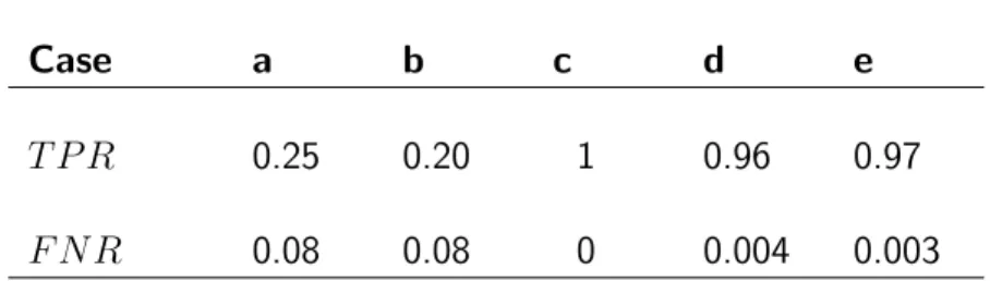
for each method on yarn data. . . 59 4.1 The true positive rate (T P R) and the false negative rate (F N R)

2.1 Estimation picture for LASSO (left) and ridge regression (right). Shown are contours of the error and constraint functions. The solid blue areas are the constraint regions |β1|+|β2| ≤ t and β12+β22 ≤ t2, respec-tively, while the red ellipses are the contours of the least squares error function [Tibshirani (1996)]. . . 17 3.1 PCR and PLSR schematic representation. The left hand plot shows

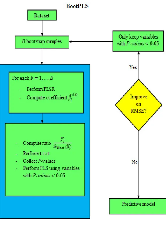
the first stage of the bilinear model. The red arrows represent the direction of the first 2 components. The general process of PCR and PLSR are illustrated in the right plot. . . 30 3.2 Flowchart summarizes BootPLS algorithm. . . 50 3.3 Comparison between the predictive ability of PLSR, PCR, JKPLS,

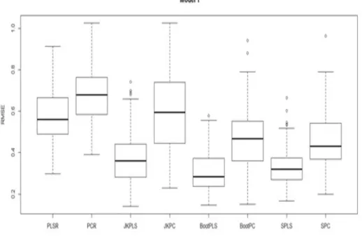
JKPC, BootPLS, BootPC, SPLS, and SPC for Model 1. . . 55 3.4 Comparison between the predictive ability of PLSR, PCR, JKPLS,

JKPC, BootPLS, BootPC, SPLS, and SPC for Model 2. . . 56 3.5 Comparison between the predictive ability of PLSR, PCR, JKPLS,

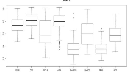
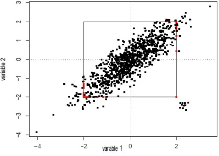
JKPC, BootPLS, BootPC, SPLS, and SPC for Model 3. . . 56 4.1 Limitation of separate univariate winsorizations (c = 2). The

corre-lation outliers (red points) are only shrunken to the boundary of the square(Khan et al. (2007)). . . 69

1

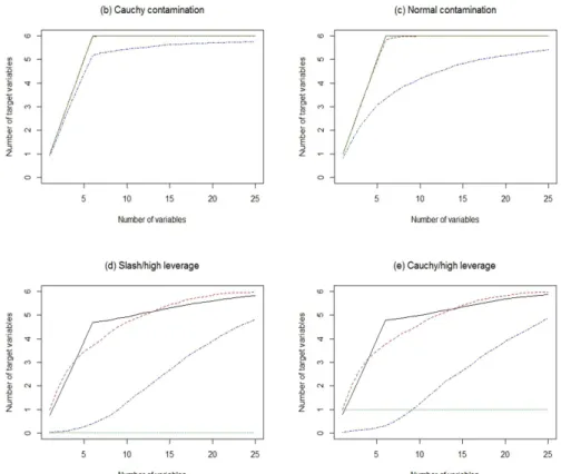
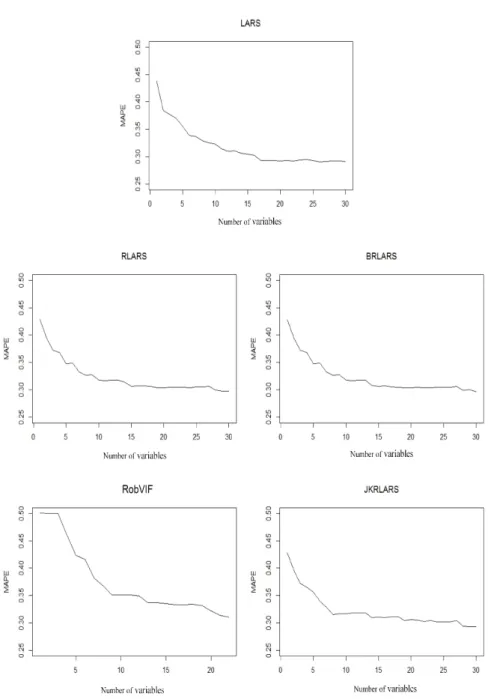
4.3 Average number of target variables tm versus m for LARS, RLARS, RobVIF, and JKRLARS for scenarios (a)-(e). The lines shown in all plots follow the legend of figure (a). . . 80 4.4 Learning curves for LARS, RLARS, BRLARS, RobVIF, and JKRLARS

on Census data. Each learning curve suggests the optimal number of predictors for each method. . . 83 4.5 Box plots of MAPE values of the optimal number of selected variables

Introduction

Regression models have been widely used in many different areas such as health, biology, environment, management, and etc. Motivated by various applications, there has been a dramatic growth in the automated means of data collection, yielding data sets with a huge number of observations and larger numbers of potentially relevant predictor variables than before.

Usually, there are some correlated predictor variables, and including all of them in a statistical model will not necessarily improve the model’s prediction performance. On the other hand, the interpretation of models with fewer predictors is easier and more tractable than for models with a large number of predictors. Therefore, finding the best variables among all candidate predictor variables is an important and challenging problem to study.

When the data contains atypical observations such as outliers, we need a robust vari-able selection method that is resistant to outliers in order to select varivari-ables reliably. In this situation, when the data contains atypical observations, outlier detection and variable selection are inseparable problems. Therefore, a robust method that can si-multaneously detect outliers and select variables is needed.

ˆ selecting the relevant predictor variables for regression models with large number of predictors;

ˆ detecting outliers and robustly selecting the relevant predictor variables in the presence of outliers in data sets with large number of predictors.

Given that there are some regression methods which are well-known and popular to reduce the dimension of the data but still requiring the elimination of irrelevant pre-dictor variables, we plan to present a variable selection procedure for these regression methods in the presence of large number of predictor variables in data.

We will also present an outlier detection and robust variable selection method using computationally efficient regression methods in dealing with contaminated data sets with large number of predictors.

1.1

Variable Selection

Consider the design matrix X = [1 x1. . .xp] with p predictor variables and a response variabley, withnobservations, the classical linear regression model supposes

y=Xβ+e, (1.1)

with parametersβ= [β0, β1, . . . , βp]T. The errorse= [e1, e2, . . . , en]T are assumed to haveE(e) = 0andvar(e) =σ2_{I, whereIis the identity matrix. We aim to select} the relevant predictor variables to entering the regression model.

In the variable selection problem, there is uncertainty as to which subset of predictor variables to use. This problem receives more attention especially when the number of variables p is large and there are irrelevant and/or redundant variables in the set of predictors. For fitting the regression model (1.1), which is as follows

ˆ

where

ˆ

β = XTX−1

XTy (1.3)

a variable selection technique should identify which subset of p predictors truly have nonzero coefficients and which have zero coefficients. In order to build an accurate linear predictor of type (1.2), we should force the coefficients of this set of variables to nonzero and the rest to zero. In data analysis, this is a fundamental problem and is not limited only to linear regression or to the field of statistics.

1.1.1

Need for Variable Selection

There are several advantages in using an efficient variable selection algorithm. One reason is simplicity and interpretability. In order to understand the functional relation between the response variable (output) and the predictor variables, finding the most relevant and potential predictor variables leads to the dimension reduction of the number of variables and to a simpler interpretation and understanding of the model.

The next reason is saving time. The best subset selection methods involve considering all possible subsets of candidate predictors for calculating a suitable model. These methods are also difficult to apply to data sets with large number of predictors. For instance, withp number of predictor variables2p _{different models should be tried for} an extensive search of all possible subsets, and therefore considering all of these models is very time-consuming. (Kadane and Lazar (2004)). Thus, an efficient algorithm can save a lot of time and also the costs of finding the true model out of a large number of models.

The other reason is prediction performance, which can be improved by selecting the true predictors (i.e., those predictors whose regression coefficients are nonzero). In fitting the models using least squares regression, adding each new predictors to the model adds to the variance of the predicted values. Hence, the fewer the number

of estimated coefficients the lower the variance. By using efficient variable selection methods, we can be confident to select the correct number of variables small enough to have a small variance, but large enough to yield a good prediction performance (see details in Hastieet al. (2009), Miller (2012)).

1.2

Outlier Detection and Robust Variable

Selec-tion

If the errors in the classical linear regression model (1.1) follow a mixture distri-bution, for instance a mixture of Normal distribution and some general distribution

F, that is e∼(1−a)N(0, σ2_{) +aF, where 0< a≤1, then they do not follow the} assumptions of the classical linear regression model. Variable selection problem has not been studied well in these situations, and most of the variable selection methods use least squares in some way. Many estimation procedures like least squares can be highly effected by a small proportion of outliers in data. Hence, robust variable selection methods are needed to remedy this problem and do show a reliable behavior in the presence of outliers in data. In contaminated data sets, outlier detection and variable selection are not two separable things since selection may have effects on what is considered as an outlier and vice versa.

1.3

Thesis Overview

1.3.1

Objectives and Achievements

In this thesis we develop principal components regression (PCR) and partial least squares regression (PLSR) as two popular regression methods to enable them for variable selection (Massy (1965), Helland (1988), Helland (1990), Zou et al.(2006), Chunget al. (2013)).

We evaluate and compare the performance of the proposed methods with their coun-terparts on both different simulation studies and real data sets. The proposed variable selection algorithm for both PCR and PLSR is competitive with its counterparts pre-sented in the literature review or even outperforms them according to the considered simulation studies. The application of the methods on real data also confirms the good performance of the proposed variable selection algorithms (Shahriari et al.

(2014)).

We also aim to develop and enable the powerful modified version of the forward stage-wise procedure to perform outlier detection and robust variable selection simul-taneously (Efronet al. (2004), Khanet al. (2007)). We investigate and compare the performance of the proposed outlier detection and robust variable selection method on both simulated and real data sets. This method presents a robust version of the classical least angle regression (LARS) (Efronet al. (2004)) and is competitive with its counterparts presented in literature review or even outperforms them (Shahriari

et al. (2014)).

1.3.2

Variable Selection Ability

We contribute with variable selection algorithms for principal components regres-sion (PCR) (Massy (1965)) and partial least squares regresregres-sion (PLSR) (Helland (1988), Helland (1990)) as two popular applicable high-dimensional regression meth-ods (i.e., regression methmeth-ods that can be used even when p n). The basic idea of these algorithms is based on the significance tests of the regression coefficients in the PCR/PLSR model. This technique automatically generates a standard error estimates of the coefficients parameters and then, by dividing the estimated regres-sion coefficients by their estimated standard errors, the t-test values will be obtained, giving the significance level for each parameter. The estimated regression coefficients are calculated using bootstrap (Efron (1982)). Based on such bootstrap estimates of

the regression coefficients, useless variables may be eliminated automatically in order to simplify the model, which makes it more reliable. This approach enables PCR and PLSR to perform variable selection.

By conducting different simulation studies, the proposed method is evaluated and compared with its counterparts presented in the literature review. The results of dif-ferent simulation scenarios showed that the performance of the proposed method is competitive or outperforms in the considered simulation studies in comparison with its counterparts. We also applied the methods to real data and the results yielded the same achievements in simulation study.

1.3.3

Outlier Detection and Robust Variable Selection

Devel-opment

We present an algorithm for the least angle regression (LARS) (Efronet al.(2004)) which is a modified version of the forward stage-wise procedure. The LARS algorithm is a powerful and computationally efficient method to sequence the predictor variables for least squares regression. Since LARS is based on the pairwise correlation between the predictor variables and the response variable, it is not robust to the presence of a small amount of anomalies in data. We propose a method capable of outlier detection and robust variable selection simultaneously which presents a robust sequence of predictor variables for LARS.

This method is obtained by combining robust least angle regression with least trimmed squares regression (Rousseeuw (1984), Rousseeuw and Van Driessen (2006)) on jack-knife subsets (Efron (1982)) to detect outliers. The detected outliers are then removed to obtain the clean data, then standard least angle regression is applied on this clean data to robustly sequence the predictor variables in order of their importance.

1.3.4

Thesis Structure

The first section of this chapter consists of the description of the variable se-lection problem and its advantages for the regression models with a large number of predictors. Then we point to the problem of variable selection when the data contains outliers, thus revealing the necessity for a robust variable selection method.

The following chapters of this thesis are organized as follows. In Chapter 2, we will describe the literature related to variable selection and some popular regression meth-ods for data sets with large number of predictors.

In Chapter 3, first we will provide the methodology of principal components regression (PCR) and partial least squares regression (PLSR). We will also address why these two popular methods need to be developed to perform variable selection. Second, we will describe the existing sparse based methods for principal components regression and partial least squares regression, and then we will explain resampling methods which will be used inside our variable selection approach to produce automatic estimates for the regression parameters. Finally, we will propose variable selection algorithms to enable principal components regression and partial least squares regression in order to find the most relevant predictor variables. Different simulation scenarios will be conducted along by using real data to evaluate and to compare the performance of the mentioned methods, and the results will be discussed.

In Chapter 4, we will address the sensitivity of linear regression followed by least squares to the presence of outliers in data and will describe some popular robust vari-able selection methods which are resistant in these situations. We will point out the least angle regression and its sensitivity to the presence of outliers in data and will review the existing robust least angle regression method, as our method’s counterpart. We will also describe another robust variable selection method based on the variance inflation factor (VIF), which also inherits the spirit of a variation of forward stage-wise regression. Then, we will propose our approach for identifying outliers and robustly

selecting variables for least angle regression, simultaneously. Finally, by conducting different simulation studies we will investigate and compare the performance of the proposed method with its counterparts. We will also apply the mentioned methods to real data. The results of both simulation study and real data will be discussed. Finally, in Chapter 5, the conclusions of our study will be drawn by summarizing the main ideas and the results of this thesis, and future developments will be addressed.

Review: Variable Selection in Linear

Regression

2.1

Introduction

The method of least squares (LS) is a standard approach to estimate the param-eters in regression analysis. LS minimizes the sum of squared errors, in a regression model. There are two main reasons why we are often not convinced with least squares estimates:

ˆ Predictive ability: least squares estimates has low bias (zero bias) but suffers from high variance. Therefore, it may be worth sacrificing some bias to reduce the variance of the predicted values, and, as a consequent, to increase the model’s predictive ability. This can be achieved by shrinking or setting some coefficients to zero (Hastie et al. (2009), Miller (2012));

ˆ Interpretation: it can be helpful to determine a smaller subset of variables through a large number of predictor variables in order to simplify the model for interpretation.

As we represented in Section 1.1 in Chapter 1, our aim is to select the most relevant predictor variables in linear regression models. The selection criteria are numerous and can be based on prediction, fit, and etc. We define some notation in order to explain these selection criteria.

Suppose we are fitting a model, which we call submodel, with a subset of the possible predictor variables. We define qsubmodel as the number of variables in the submodel plus one for the intercept, which is the number of nonzero coefficients we would fit in this model. When we use least squares to predict the response variable, given the submodel, we name this prediction,yˆ_submodel.

We define the total sum of squares,SSTsubmodel = n

P

i=1

(yi−y¯)2, withy¯the mean of the response variable, the regression sum of squares,SSRsubmodel =

n

P

i=1

(ˆysubmodel,i−y¯)2, the residual sum of squares, RSSsubmodel =

n

P

i=1

(yi−yˆsubmodel,i)2, and the hat matrix

H =X(XXT₎−1_XT _{for the full model which contains p predictors plus one for the} intercept.

One simple idea in full model is to use adjustedR2 _{which adjusts the multiple} corre-lation coefficient for the number of parameters fitted in the model withn number of observations R_adj2 = 1− n−1 n−qsubmodel−1 (1−R2), (2.1) where R2 ₌ SSRsubmodel SSTsubmodel = 1−RSSsubmodel SSTsubmodel .

A related criterion is Mallow’sCp statistic (Mallows (1973)). For a given model where we fitqsubmodel parameters,

Cp =

RSSsubmodel ˆ

whereσˆ2 ₌ RSSf ull

n−p−1, where pis the number of predictors, and RSSf ull = n

P

i=1 (yi− ˆ

yi)2. The motivation behind Cp was to create a statistic to estimate the mean square prediction error (Mallows (1995)).

Some other selection criteria, such as akaike information criterion (AIC), and the correctedAIC (AICc) (Akaike (1970), Akaike (1974), Sugiura (1978)) are as follows

AIC =nlog(RSSsubmodel

n ) + 2qsubmodel; AICc =nlog( RSSsubmodel n ) + 2(qsubmodel+ 1)× n (n−qsubmodel−2) .

Cp,AIC, andAICctend to select too large of a subset and the data is overfit (Shao (1993)).

The existing selection procedures can be broadly categorized into three classes ac-cording to their general strategy and respective computational efficiency.

A first class considers the potential subsets of predictors. All possible subset selection

considers all the combination subsets of the predictors and evaluates each of these submodels according to a fixed criterion. The model which best satisfies the selection criteria is chosen as the optimal model. Stepwise subset selection is built on the basis of sequential selection procedures in which a predictor at a time is added to (or removed from) the model, based on a criterion that can change from one step to the next and that is calculated for all potential predictor variables to add (or to exit) until another criterion is satisfied. The second class shrinks the regression coefficients by imposing a penalized term on their size in order to satisfy bias to reduce the variance of the predicted values, and, as a consequent, to increase the model’s predictive abil-ity. The third class of selection procedures is also formed of sequential procedures in which each predictor is evaluated to enter into a model as a potential predictor. Each predictor is evaluated once to enter as a potential predictor.

The selection criteria such asAIC, AICc (Akaike (1970), Akaike (1974)), Mallow’s

into the first class. When the numberp of the predictor variables is small, one may compute these selection criteria for all possible subsets of predictors. But as the num-ber p of the predictor variables increases, the number of subsets grows dramatically; as a result, the computational burden of using this approach is increased and makes it infeasible for computation. This problem leads to the popularity of step-by-step algorithms like forward selection and stepwise (SW) selection procedures (Weisberg (2014)).

The second class may contain shrinkage methods in which the estimator of the re-gression coefficientsβ minimizes the sum of squared errors according to a norm q as a penalized term, i.e.,

arg min β n ky−Xβk2₂+λqkβk q q o , (2.3)

whereX = [1 xj]j=1,...,p with1 a column of ones, kβkq = p P j=1 |βj|q !1/q forq >0, andkβk0 = p P j=1

I{βj6=0} withI{βj6=0} = 1ifβj 6= 0and 0 otherwise (Linet al.(2011)).

Shrinkage methods that useq = 1norm penalization are least absolute shrinkage and selection operator (LASSO) (Tibshirani (1996)), and the Dantzig selector (Candes and Tao (2007)). Ridge regression is another shrinkage method which uses q = 2 norm penalization.

The third class may include a variation of the stepwise regression that evaluates predictors sequentially. Least angle regression (LARS) (Efron et al. (2004)) can be categorized into this class. Streamwise regression (Zhou et al. (2006)), which evalu-ates predictors sequentially, though each of them is considered once to enter to the model, can also be categorized into this class. This approach uses the α-investing rule (Foster and Stine (2008)) and is a fast procedure.

Variance inflation factor (VIF) is an improved streamwise regression approach where the selected model is given by computing a fast test statistic based on the variance

inflation factor of the candidate variable (Lin et al. (2011)).

In Section 2.2 of this chapter we will describe all possible subset selection proce-dures, along with some classical step-by-step algorithms, such as forward stepwise and backward elimination selection. In Section 2.3 some popular shrinkage methods such as ridge regression and least absolute shrinkage and selection operator (LASSO) will be reviewed. Finally, in Section 2.4 the modified versions of stagewise regression, least angle regression (LARS) and variance inflation factor (VIF) regression will be described.

2.2

Potential Subset Selection

In subset selection only a subset of variables is kept and the rest of them is removed from the model. The coefficients of the potential predictors as the inputs of the model are estimated using least squares regression. There are a number of different strategies for subset selection.

2.2.1

All Possible Subset Selection

This approach considers all 2p possible subsets of the predictor variables and determines the subset of the predictors of a given size that maximizes a measure of fit or minimizes an information criterion based on a monotone function of the residual sum of squares. The efficient algorithm ”simple leap and bound”(Furnival and Wilson (1974)) can find the best subsets without examining all possible subsets. With a fixed number of terms in the regression model, there are a number of criteria such as the

AIC (Akaike (1970)), Mallow’s Cp (Mallows (1973)) that one may use to evaluate a subset of predictor variables; typically we choose the smallest model that minimizes the residual sum of squares. So, for instance, if a subset with a fixed number of terms satisfies a criteria among all subsets of sizek, then this subset will also satisfies other

selection criteria among all subsets of fixed size k. This process is not feasible for a large number p of predictor variables, and this problem leads to the popularity of step-by-step algorithms.

2.2.2

Forward Stepwise and Backward Elimination Selection

As we mentioned before, finding the best model among all the possible submodels will become infeasible whenpis large. Therefore, in order to decrease the computation time we can search through all possible subsets to find a good path through them. In this section, we review some of the most important of this kind of algorithms. Forward stepwise selection starts with all coefficients equal to zero, and then sequentially adds to the model the predictor that most improves the fit (in the other words, the predictor that minimizes the criterion of interest or if an information criterion is used, then this amounts to find the most correlated predictor with the response variable). The procedure is continued until all predictors have been added to the model.

Backward elimination selection starts with the full model and at each step drops a predictor with the least impact on the fit; therefore it is the opposite of forward stepwise selection procedure. The procedure is continued until all predictors have been deleted from the model (Weisberg (2014)).

2.2.3

Forward Stagewise Regression

Forward stagewise (FS) regression is similar to forward stepwise regression but it is more constrained (Hastieet al.(2009)). It starts like forward stepwise regression with an intercept equal to y¯, with all coefficients equal to zero. At each step, the most correlated variable with the current residual enters into the model. Then, the simple linear regression coefficient of the residual on this selected variable is estimated and then added to the current coefficient for that variable. This process is continued until none of the variables have correlation with the residuals. Since none of the variables

is adjusted when a predictor is entered into the model, therefore it can take many steps in the direction of the same predictor in order to reach the least squares fit.

2.3

Shrinkage Methods

In subset selection procedure, a subset of the predictor variables is kept and the rest are removed; as a result, a model that is interpretable with lower prediction error than the full model is obtained. But since this procedure proceeds in a discreet way, i.e. variables are either kept or removed, it often shows high variance, and so does not reduce the prediction error of the full model. Shrinkage methods are more continuous, and do not suffer as much from high variability (Hastie et al. (2009)).

2.3.1

Ridge Regression

Ridge regression (Hoerl and Kennard (1970)) shrinks regression coefficients by penalizing their size. The ridge estimates minimize a penalized residual sum of squares,

ˆ

βridge = arg min

β ( _n X i=1 (yi−xTi β) 2 +λ p X j=1 β_j2 ) = arg min β ky−Xβk2₂+λkβk2₂ (2.4) Here λ ≥0 is a penalty parameter which controls the amount of shrinkage; i.e. the larger the value of λ, the greater the amount of shrinkage. When λ = 0, we get the least squares estimates; when λ ' ∞, we get βˆridge = 0; when λ is between these two values, we are balancing two ideas: fitting the linear regression model, and shrinking the coefficients.

An equivalent form of writing the ridge problem is

ˆ

βridge = arg min

β (y−Xβ)2, (2.5) subject to p P j=1 β2 j ≤t, where t is a tuning parameter varied over a certain range.

This rewriting form makes explicit how ridge regression puts constraint on the size of the parameters. Parameter λ in (2.4) has a one-to-one correspondence with t in (2.5).

In the presence of many correlated variables in a linear regression model, their co-efficients can become poorly determined and show high variance. One variable with a large positive coefficient can be canceled by a similarly negative coefficient as its correlated cousin. Imposing a constraint on the size of the coefficients, as in (2.5), this problem is thus conciliated. It should be noticed that the intercept term has left out the penalty term, the solution forβˆ0 = ¯y, and so we assume that the inputs have been standardized before solving (2.4).

2.3.2

Least Absolute Shrinkage and Selection Operator

Least absolute shrinkage and selection operator (LASSO) (Tibshirani (1996)) shrinks the regression coefficients by imposing norm 1 as the penalty parameter. LASSO is like ridge regression but the penalty term is kβk₁ instead of kβk₂ as in ridge regression. The LASSO estimate is defined as

ˆ

βlasso= arg min

β ( n P i=1 (yi−xTi β)2+λ p P j=1 |βj| ) = arg min β n ky−Xβk2₂+λPp j=1|βj| o = arg min β ky−Xβk2₂+λkβk₁ . (2.6)

Figure 2.1: Estimation picture for LASSO (left) and ridge regression (right). Shown are contours of the error and constraint functions. The solid blue areas are the constraint regions|β1|+|β2| ≤tandβ12+β22 ≤t2, respectively, while

the red ellipses are the contours of the least squares error function [Tibshirani (1996)].

Just as in ridge regression, we can rewrite (2.6) as

ˆ

βlasso= arg min

β (y−Xβ)2, (2.7) subject to p P j=1 |βj| ≤t,

where t is a tuning parameter over a certain range.

Because of using q = 1 norm penalization as you can see in Figure 2.1, LASSO can shrink the regression coefficients exactly to zero, and therefore can perform vari-able selection. The LASSO estimator can be computed using the efficient least angle regression algorithm (LARS), which is a modified version of forward stagewise proce-dure. Like ridge regression, the inputs are standardized and the solution forβˆ0 = ¯y, and thereafter we fit a model without an intercept.

LASSO and Ridge Regression As we mentioned in Section 2.3.1, when there are many correlated variables in a linear regression model, the estimates may exhibit high variance. Ridge regression, by imposing a restriction on the size of the regression coefficients, tries to alleviate this problem.

Ridge regression shrinks the regression coefficient toward zero but is not able to set some coefficients exactly equal to zero; thus, unlike LASSO, cannot perform variable selection.

2.4

Modified Versions of Stepwise Regression

In this section we describe two modified and improved versions of stepwise re-gression which are fast to compute and sequence the predictor variables in their importance.

2.4.1

Least Angle Regression

Least angle regression (LARS) (Efronet al. (2004)) enters variables in the model in order of their importance. LARS is related to forward stagewise (FS) procedure, which sequentially adds variables to the model in small steps. FS uses in each step the most correlated variable with the residuals, and updates the fit by adding only a small fraction of the least squares contribution of this variable to the model. Usually, FS takes a large number of steps using the same variable before another variable yields a higher correlation with the remaining residual. Therefore, FS is not computationally efficient. By deriving a simple mathematical formula for the optimal step size of a selected variable, LARS largely reduces the number of steps and speeds up the computation time.

The steps of the LARS algorithm can be summarized as follows:

to response vector y;

2. Find the predictor that is most correlated with the response variable, say x1;

3. Take the largest step possible in the direction of this predictor until some other predictor, sayx2, has the same maximal correlation (in an absolute value) with the current residual;

4. Proceed in the equiangular direction of the two predictors until a third variable

x3 earns its way into the ”most correlated”set. The equiangular direction is the

direction in which the correlation of the predictors decreases at the same pace so that these correlations remain equal at all times;

5. Repeat until all predictors have been entered.

LARS is only based on the means, variances and correlations of the data, and so it is sensitive to the presence of contamination in the data. In Chapter 4 we will discuss about its sensitivity and to remedy this problem we will present a robust version of this algorithm and evaluate the performance of our method against its counterparts.

LARS and LASSO LARS and LASSO are closely connected. LARS can provide an

efficient algorithm to compute the LASSO path. By modifying the LARS algorithm, the LASSO path can be obtained as follows: if a non-zero coefficient crosses zero, remove its variable from the active set of variables and recompute the best direction, that is, current joint least squares direction.

2.4.2

Variance Inflation Factor (VIF)

Variance inflation factor (VIF) regression (Linet al. (2011)) also inherits the spirit of a variation of stepwise regression. VIF regression searches over the predictor vari-ables to test each potential predictor variable for addition to the model. VIF regression

selects those predictors among other available predictors that can reduce a statistically sufficient part of the variance in the predictive model. VIF regression approximates the partial correlation of each candidate variable with response variable by correcting (using VIF) the marginal correlations.

The characteristics of the VIF algorithm are the following two components:

ˆ Evaluation step: the partial correlation of each candidate variable xj, j =

1, . . . , p, with the response variable y is approximated by correcting (using

the variance inflation factor) the marginal correlation using a small presampled set of data;

ˆ Search step: each variable is tested sequentially using anα-investing rule (Fos-ter and Stine (2008)). The α-investing rule purveys high accurate models and guarantees no model overfitting.

Let XS be the design matrix that contains the selected variables at stage S, and ˜

XS = [XS zj] with zj the new candidate to be evaluated for inclusion. Consider

the following models:

y=XSβS +zjβj +estep, estep∼N(0, σ2stepI), (2.8)

rS =zjγj +estage, estage ∼N(0, σstage2 I), (2.9) where rS = I−XS(XTSXS)−1XTS

y are the residuals of the fit of y on XS, I is

the identity matrix,β_S are slope parameters, and γj is the slope parameter of the fit ofzj on the residuals rS.

When there are some collinear predictors in the data, all known estimators of param-etersβj, σstep2 , and γj, σstage2 will provide different estimates and, as a consequent, significance tests based on estimates ofβj or γj do not necessarily lead to the same conclusions. While in stepwise regression the significance of βj in model (2.8) is at the core of the selection procedure, in VIF regression it is more convenient to estimate

γj.

When least squares (LS) are used to estimate,

ˆ

γj =ρ2βˆj, (2.10)

where ρ2 = zT_j I−XS XTSXS

−1

XT_Szj Lin et al. (2011). Then, a t-statistic

Tγj =

ˆ

γj

ˆ

ρσˆ with proper estimates for ρ and σ is computed and compared to the standard normal distribution to decide whether or not zj should be entered to the current model. This procedure is named VIF regression because1/ρis called the VIF forzj (see Marquaridt (1970)).

Test statisticTγj is very sensitive to outliers since it is based on the following:

ˆ the LS estimator γˆj;

ˆ ρ, in turn based on the design matrix XS and zj;

ˆ the classical estimator of σ, a form of the model deviation.

In Chapter 4 we will describe the robust version of this method and discuss its per-formance in different simulation scenarios as well as on real data.

2.5

Discussion and Conclusions

All possible subset selection procedure which seeks through all possible2p _subsets

of the predictor variables in order to find the best subset of a given size, which max-imizes a measure of fit or minmax-imizes an information criterion based on a monotone

function of the residual sum of squares, is not computationally efficient, and will be infeasible when the numberp of the predictor variables is large.

Forward stepwise selection is a greedy algorithm which produces a nested sequence of models, therefore in this sense it might seem suboptimal compared to all possible subset selection procedure. But there are two main reasons why forward stepwise selection procedure might be preferred rather than all possible subset selection pro-cedure:

ˆ Computationally: when the number p of the predictor variables is large it is not feasible to compute the best subset sequence; however, forward stepwise selection can always compute the best subset (even when p n, n is the number of observations);

ˆ Statistically: a cost is paid in variance for determining the best subset of each size; forward stepwise is a more constrained search, with lower variance but perhaps more bias.

The drawback of backward stepwise selection in comparison with forward stepwise is that it can only be used when n > p, while the later can be used at all times. In forward stagewise, unlike forward stepwise regression, none of the variables are adjusted when a term is entered to the model, and therefore forward stagewise takes many more thanp steps to achieve the least squares fit.

By keeping a subset of the predictor variables and dropping the rest, subset selection produces an interpretable model which has lower prediction error compared to the full model. However, since it proceeds in a discrete path, that is, variables are either kept or dropped, therefore it does not reduce the prediction error of the full model. Shrinkage methods are more continuous, and are not affected as much by high vari-ability.

Ridge regression does a proportional shrinkage in order to shrink the regression coef-ficients toward zero but does not set them exactly equal to zero. LASSO performs

variable selection by setting the predictor variables exactly equal to zero.

LARS and VIF regression inherit the spirit of a variation of stepwise regression. These methods are sensitive when data contains outliers, and in Chapter 4 we will discuss their sensitivity to outliers.

Sparsity for Principal Component

and Partial Least Squares

Regression

3.1

Introduction

High-dimensional regression (regression analysis when the number of predictors is larger than the number of observations) has captured the attention of many statis-ticians worldwide, because of its interesting applications, as well as the unique chal-lenges faced. Motivated by interesting applications, there has been a dramatic growth in the development of statistical methodology in the analysis of high-dimensional data (p n), particularly related to regression (model selection, estimation and predic-tion).

The problem of high-dimensional variable selection has received tremendous atten-tion during the last decades because variable selecatten-tion plays an important role in high-dimensional statistical modeling (Fan and Li (2001) and Linet al. (2011) among many others). The usual variable selection procedure using least squares and a penalty

which involves the number of parameters in the candidate submodel (e.g. AIC) is infeasible to compute exhaustively (B¨uhlmann and Van de Geer (2011)). Forward selection strategies are computationally fast but they can be very instable, yielding poor results (Breiman (1996)). Best subset selection methods involve considering all possible subsets of candidate predictors for calculating a suitable model. These methods are also difficult to apply to high dimensional data. For instance, if the number of predictors is p, then 2p _{different models should be tried for an} exten-sive search of all possible subsets. This value, even for moderate values of p, grows exponentially and makes the search impractical (Trevoret al. (2001)). Although sev-eral search-based strategies such as artificial neural network (Burden et al. (1997)) and genetic algorithms (Jouan-Rimbaudet al.(1995)) have been successfully applied to variable selection problems, these methods still have some drawbacks. Several variable selection (VS) methods in high dimensional data in the unified framework of penalized likelihood estimator are ridge regression (Frank and Friedman (1993)), LASSO (Tibshirani (1996)), elastic net (Zou and Hastie (2005)), the new smoothed LASSO (Meier and B¨uhlmann (2007)) and boosting algorithms (Fan and Lv (2010) and B¨uhlmann and Van de Geer (2011)).

Principal components regression (PCR) and partial least squares regression (PLSR) are well-known techniques in dealing with high-dimensional data whose number of pre-dictorsp is larger than sample sizen (Engelenet al. (2004), Helland (1988), Helland (1990) and Hubert and Verboven (2003)). PCR (Massy (1965)) and PLSR (Wold (1966)) are two related families of methods that contain selecting a subspace of the column space of the predictors on which to project the response vector. These meth-ods latter appeared in chemometrics, sensory evaluation and food research (Wold (1975b), Wold et al. (1984), Geladi and Kowalski (1986), Martens and Martens (2000), Martens and Næs (1989), Stone and Brooks (1990), and De Jong (1993b)). PCR and PLSR as two dimension reduction techniques that have recently obtained much attention in high dimensional genomic data (Boulesteix and Strimmer (2007)).

Although PCR and PLSR are two popular techniques that can handle multicollinearity among predictors even when there are more predictors than observations, it is still necessary to eliminate irrelevant predictors in high-dimensional data. The drawback of PCR and PLSR is that, when using these two methods, the number of variables used is not reduced, since the components are linear combinations of all the predictors. This drawback makes it often difficult to interpret the derived principal components (PC). In order to help practitioners to interpret principal components, rotation tech-niques are commonly used (Jolliffe (1995)). There is a technique which restricts the loadings in principal components to take values from a small set of given integers such as 0, 1, -1 (Vines (2000)).

Existing irrelevant variables can influence the PCR and PLSR models. Imposing spar-sity in the midst of dimension reduction step may lead to variable selection. Huang et al. (2004) recently proposed a penalized PLS method that thresholds the final PLS estimator (Huang et al. (2004)). Chun and Kele¸s (2010) formulated sparse partial least squares (SPLS) regression by relating it to sparse principal component analysis (SPCA) (Jolliffe et al. (2003), Zou et al. (2006)). SPCA involves formulating prin-cipal component (PC) analysis as a regression-type optimization problem, and then obtaining sparse loadings by imposing LASSO (Tibshirani (1996)) (and a generaliza-tion of LASSO, elastic net) constraint on the regression coefficients. Therefore, it is important to reduce the size of the explicitly used variables (i.e., variable selection) besides having dimension reduction for PCR and PLSR. We introduce an approach which is based on bootstrap technique for significance tests of the regression coeffi-cients to perform variable selection inside PCR and PLSR.

The rest of this chapter is organized as follows. First, in Section 3.2 we will give an introduction of the methodology for PCR and PLSR, and will compare PCR and PLSR. Then, in Section 3.3 we will review jack-knife and bootstrap as two resampling methods. We will explain some variable selection methods for PCR and PLSR, along with our proposed approach in Section 3.4. We will conduct a simulation study in

Section 3.5 to compare the performance of the presented variable selection methods for PCR and PLSR. In Section 3.6, we will show the results of the simulation study. We will also apply these methods to a real data in 3.7; and finally in Section 3.8 we will conclude.

3.2

Principal Components Regression and Partial

Least Squares Regression

As mentioned before in Section 1.1 in Chapter 1, a linear regression model assumes that there is a linear relationship between the response variable and the set of the predictor variables. There are various methods to estimate the slope parameters β

in a linear regression model. In the presence of large number of predictors in the model, LS can be used; however, if the number of predictors gets too large (more than the number of observations, p n, the matrix XTX gets singular), the corresponding multiple linear regression (MLR) model obtained by LS is not able to fit the sampled data well and simultaneously predict the new data well; that is the problem of overfitting. To remedy this problem, PCR and PLSR can be used, since they reduce the dimension of the design matrix X. Also, they can handle the multicollinearity in the data.

PCR and PLSR are two multivariate regression methods concerned with explaining the variance-covariance structure of the data through a small number of components which are linear combinations of the original variables (Engelen et al. (2004)). The basis of both techniques is a bilinear model that explains the existence of a relation between a set ofp-dimensional predictors and a response variable through the latent component matrix Tn×k = (t1, . . . ,tk) where the ti, i = 1, . . . , k are the score

vectors, withk p. By considering the observations(X,y), we assume that,

X =1x¯+T PT +ν, (3.1)

y=1y¯+T q+ξ. (3.2)

Here x¯ is the p-dimensional mean vector of predictors, y¯ the mean of the response variable, P the p×k matrix of loadings and q represents the k-component slope parameters in the regression ofyon theti. The error terms are denoted by then×p matrix ν and the vector ξ with n elements. These corresponding errors show the unique variation inX and ythat is not explained by thek-component bilinear struc-ture. The errors may be due to operator mistakes, measurement noise, mis-specified model, etc. In order to make inference on the ordinary least squares estimator of q, an assumption on the errors ofξ ∼N(0, σ2I)is needed. This condition is equivalent to assuming y|q ∼ N(1y¯+Tq, σ2_{I) which represents that the variance-covariance} matrix of y depends only on one parameter σ2; such a matrix is also known as a scalar covariance matrix.

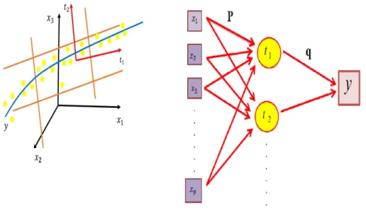
Figure 3.1 shows the major two stages of PCR and PLSR. In the first step, due to (3.1), the latent componentstiare built as linear combinations of the original predictor

variables or, in the other words, the high-dimensional observationsX are summarized in latent componentstis of dimensionkp. The model’s predictive ability depends on the numberk of components selected. If too few components are chosen, the valid structure in the data is left and the model under-fits the data. Choosing too many components will lead to over-fitting in the data, pulling too much noise which will diminish model prediction. Various different criteria (such as AdjustedR2_{, root mean} squared error (RM SE)) can be used in order to select the number of componentsk

(Aucott et al. (2000)). Cross-validation (CV) or independent test set validation are usually applied to select the optimal number of components. If the amount of existing

Figure 3.1: PCR and PLSR schematic representation. The left hand plot shows the first stage of the bilinear model. The red arrows represent the direction of the first 2 components. The general process of PCR and PLSR are illustrated in the right plot.

data is limited, especially for high-dimensional data, cross-validation is preferable to independent test set validation (Martens and Næs (1989)).

For the second step of the algorithm, due to (3.2), these k latent components will become the regressors for the y. The objective of the second step is to find a

k-dimensional regression hyperplane that best fits the data (y,Tn×k). At last, the estimates for the parameters of the original predictor variables, βˆ, can be obtained from the bilinear model.

A large body of literature has compared PCR and PLSR (Martens and Næs (1989), Stone and Brooks (1990), Wentzell and Vega Montoto (2003), Schumann et al.

(2013)). Both methods construct new predictors, known as components, as linear combinations of the original predictors, but they construct those components in differ-ent ways. The construction of thek-dimensional scores vector ti by PCR and PLSR

is not the same. PCR creates components to explain the observed variability in the predictors, without considering the response variable at all, and thus using a variance criterion. On the other hand, PLSR does take the response variable into account, and therefore often leads to models that are able to fit the response variable with fewer components, i.e., PLSR finds linear combinations of the predictors that best explain the response by maximizing a covariance criterion between the predictors and the response variable (Frank (1987), Næs et al. (2002)). With the same number of latent variables, PLSR will cover more of the variation in response variable and PCR will cover more variation of the original predictor variables.

In practice, however, there is hardly any difference between the use of PCR and PLSR; by construction, it is thus expected that PLSR requires less components than PCR (Frank and Friedman (1993), Mevik and Wehrens (2007)). In most situations, both methods achieve similar prediction performances, although by construction it is expected that PLSR gives improved prediction results with fewer components than PCR (De Jong (1993a), Garthwaite (1994)). Some components from a PCR model fit may serve primarily to describe the variation in the predictors, and may include large weights for variables that are not strongly correlated with the response. Thus, PCR can lead to retaining variables that are unnecessary for prediction.

3.2.1

Principal Components Regression Algorithm

Principal component analysis (PCA) is a popular statistical method which can ex-plain the covariance structure of the data through a small number of components which are linear combinations of the original predictor variables (Jolliffe (2005)). These components can be used for an interpretation and a better understanding of the different sources of variation. PCR is based on principal component analysis. PCR preforms a least-squares regression of projections of data onto the basis vectors of a factor space (Kramer (1998)). In PCR, instead of directly regressing the response

variable on the predictor variables, the principal components are used as regressors. One typically uses only a subset of all the principal components for regression. Often the principal components with higher variances (those that are based on eigenvectors corresponding to the higher eigenvalues of the sample variance-covariance matrix of the predictors) are chosen as regressors. However, for predicting the response vari-able, the principal components with low variances may also be important, and in some cases even more important (Jolliffe (1982)). In the classical approach, the first component corresponds to the direction in which the projected observations have the largest variance. The second component is then orthogonal to the first and again maximizes the variance of the data points projected onto it. Proceeding in this way produces all the principal components, which correspond to the eigenvectors of the empirical covariance matrix.

First, PCR centers the data using the column mean x¯ of the x-variables and the meany¯of the y-variable. Denote the centered observations by

˜

X =X −1x¯, ˜

y=y−1y¯.

Then, for dealing with the multicollinearity in the x-variables, the first k (k ≤

min(n, p)) principal components of X are calculated. These loading vectors Pˆ =

(ˆp₁, . . . ,pˆ_k) are the k eigenvectors that correspond to the k largest eigenvalues of

the empirical covariance matrix Sx =

1

n−1

˜

XTX˜ (Jolliffe (1982), Jolliffe (2005)).

Therefore, these loading vectors are uncorrelated, orthogonal and they construct a new coordinate system in the k-dimensional subspace that they span. Denote the eigenvalues of the Sx, by τˆ1, . . . ,τˆp. The sums-of-squares of the component scores

ˆ_{t1, . . . ,}ˆ_{tp are calculated as τˆa = ˆt}T

aˆta, a = 1, . . . , p. The orthogonality properties of

ˆ

PTPˆ =I, ˆ

TTTˆ =diag(ˆτ1, . . . ,τˆk),

where I is the identity matrix and diag() denotes a diagonal matrix with zero ele-ments off the leading diagonal. Then, the k-dimensional scores of each data point ˆ_{ti are calculated as the coordinates of the projections of X}˜ _{onto this subspace, or}

equivalently

ˆ

T = ˜XPˆ( ˆPTPˆ)−1 = ˜XPˆ. (3.3)

It can be shown that for centeredx-variables thepˆ_a, a= 1, . . . , k dimensional vectors are eigenvectors ofX˜TX˜ with the ˆτ’s as eigenvalues. This means that all pˆ’s satisfy the equation

˜

XTX˜pˆ_a= ˆp_aτˆa.

Likewise, it is possible to show that the scores ˆta, a = 1, . . . , k represent the corre-sponding eigenvalues ofX˜TX˜, scaled to modulus √τˆa. In the final step,ˆti are used as regressors for the centered response variable y˜. We thus fit the linear regression model using ordinary least squares as

˜

y= ˆT q+ξ,

since the data are centered, the above equation does not contain intercept. The estimated parameters are obtained as

ˆ

q = ( ˆTTTˆ)−1_TˆT_y˜,

and the fitted values

ˆ

y= ˆTˆq+1y¯

The unknown regression parameters in terms of the original variables are estimated as ˆ β_{P CR} = ˆPqˆ, ˆ β0P CR = ¯y−x¯βˆP CR. (3.4) Finally, an estimator for the variance of the errorsξ can be calculated as

Sξ = 1 n−1 n P i=1 (yi−yˆi)(yi−yˆi)T =Sy−qˆTStqˆ, (3.5) whereSy is variance ofyandStis the empirical covariance matrix of the t-variables. Note that equality (3.5) follows from the fact that the fitted values are orthogonal to the residuals (Johnson and Wichern (2002)).

For non high-dimensional data, it is possible to calculate all the positive eigenvalues and their eigenvectors simultaneously, either from the centered data X˜, or through the X˜TX˜ cross product matrix using principal components decomposition. But

the above algorithm is not proper for high-dimensional data. In such situations, PCR can be constructed with a singular value decomposition method or with the NIPALS (Nonlinear Iterative Partial Least Squares) algorithm (Wold (1966), Wold (1975a)) which is not respective to the number of observations to predictors ratio. NIPALS algorithm uses the fact that the components are orthogonal both in scores and loadings to extract one single factor at a time, a = 1, . . . , k, starting from the factor with the largest eigenvalue. We use this algorithm since it can help us to understand the PCR method. Basically, NIPALS is just an iterative algorithm based on simple least squares regressions for computing principal components. For each factor, NIPALS algorithm uses an iterative method to obtain the loading vector pˆ_a

and the score vector ˆta from the residual power-matrix (obtained after estimation of the previous a−1 factors). That initial residual matrix can be called νˆ, but for

facilitating the description of the PCA algorithm we may name itX˜a−1. It is defined by X˜a−1 = ˜X −ˆt1pˆT1 − · · · −ˆta−1pˆTa−1, where X˜ is the matrix of mean centered

X-variables. A simple algorithm for computing the a = 1, . . . , k largest eigenvalues with corresponding eigenvectors proceeds as follows

1. Choose starting values, for instance ˆta is the column in X˜a−1 which has the

largest remaining sum of squares (There are no restrictions on choosing the initial value, but choosing an appropriate initial value will speed up the conver-gence process);

2. Project the matrix X˜a−1 onˆta to improve estimate of loading vector pˆa

ˆ

pT_a = (ˆtT_aˆta)−1ˆt T aX˜a−1;

3. Normalize loading vector pˆ to length 1 in order to avoid scaling ambiguity

ˆ

p_a= _qpˆa ˆ

pT_apˆ_a ;

4. Project the matrixX˜a−1 onpˆa in order to improve estimate of scoreˆta for this

factor ˆ_{ta = ˜Xa−1pˆ} a(ˆp T apˆa) −1_;

5. Improve estimate of the eigenvalue τˆa

ˆ

τa = ˆt

T aˆta;

6. Check for convergence: if the difference between τˆa, (i.e., τˆa(new)) and the τˆa, in the previous iteration (i.e., τˆa(old)) is smaller than threshold×τˆa(new) (for instance, threshold may be 0.0001), the method has converged for this factor; if not, return to step 2.

˜

Xa= ˜Xa−1−ˆtapˆTa

and go to step 1 for the next factor. Repeat steps 2-6 until convergence. In the ideal situation, only a few eigenvalues will be large such that almost all the variation inX will be described by those first few components. One of the advantages of PCR is that it can yield good results where X-variables are highly correlated, as long as the predictive information is in the first eigenvectors. However, PCR is not effective in the following situations:

1. Since the principal components are linear combinations of the predictor vari-ables, little is achieved if these are not interpretable. In general, the predictor variables should have measurements of comparable quantities for interpretation to be possible;

2. Principal component uses only theX matrix and not the response, therefore it may happen that some low eigenvalue principal component highly contributes to the overall predictive ability of the regression model. Thus, there is no definite guarantee that PCR predicts well.

3.2.2

Partial Least Squares Regression Algorithm

Partial least squares is a family of regression based methods which combines features from principal component analysis and multiple regression. Therefore, it contains regression and classification tasks, as well as dimension reduction techniques and modeling tools. The underlying assumption of all PLS methods is that the ob-served data is generated by a system or process which is driven by a small number of latent (not directly observed or measured) variables (Rosipal and Kr¨amer (2006)). Projections of the observed data onto its latent structure by means of PLS was de-veloped by Herman Wold for econometrics ( Wold (1966)) and then applied to other fields such as chemometrics, social science, food research, etc (Wold et al. (1984),

Geladi and Kowalski (1986), Martens and Martens (2000), Hulland (1999)).

In its general form, PLS constructs orthogonal score vectors (also called latent vectors or components) by maximizing the covariance betweeny and all possible linear func-tions ofX (Frank (1987), Næs et al.(2002)). PLSR can be useful when the purpose is to predict the response and not necessarily trying to understand the underlying relationship between the predictor variables.

According to (3.1) and (3.2), the bilinear structure proceeds in two steps in PLSR algorithm. Similar to PCR, denote the mean-centered of theX and ywith X˜ andy˜,

respectively. The normalized PLSR weight vectors wa (kwak = 1) are then defined as the vectors that maximize for eacha= 1, . . . , k

cov(˜y,Xw˜ a) = ˜ yTX˜ n−1wa=Syxwa, (3.6) where ST_yx =Sxy = ˜ XTy˜

n−1 is the empirical cross-covariance matrix between the X -and y-variables. The maximization problem of (3.6) is equivalent to finding the unit weight vector wˆa that maximizes y˜TXw˜ a. For each latent variable a = 1, . . . , k, PLSR algorithm is proceeded as follows:

1. Use the variability remaining in y˜ to find the loading weight wˆa, using least

squares and the local model

˜

X = ˜ywT a +ν1

and scale the vector to modulus 1. The solution is of the form

ˆ

wa=cX˜ T

˜

y, (3.7)

where c is the scaling factor that makes the modulus of the final wˆa equal to 1, i.e.

c= (˜yTX˜X˜Ty˜)−1/2;

2. The elements of the scores ˆta are then defined as linear combinations of the

mean-centered data. It is estimated as the projection of X˜ on wˆa, i.e.,

˜

X =tawˆTa +ν2.

The least squares solution is (since wˆT_awa = 1)

ˆ_{ta = ˜Xn×pwˆa; (3.8)}

3. The loading pˆ_a is obtained from simple linear regression of the columns of X˜

onˆta, i.e.

˜

X =tapTa +ν3,

which gives the least squares solution

ˆ p_a= ˜ XTˆta ˆ_tT aˆta ; (3.9)

4. Regress y˜ onˆta to find the loading qˆa, i.e.

˜

y= ˆtaqa+ξ;

which gives the solution

ˆ qa= ˜ yT_ˆt a ˆ_tT aˆta ; (3.10)

5. Create new X˜ and y˜ matrix by subtracting the estimated effect of this factor

ˆ

ν = ˜X−ˆ_tapˆT

ˆ

ξ = ˜y−ˆ_{taqˆa. (3.12)} Note that ν1,ν2,ν3 represent different residual in steps 1-3, respectively, al-though little distinction has been made notationally. Update the formerX˜ and ˜

y by the new residuals νˆ and ξˆ, i.e. set

˜

X = ˆν, ˜

y= ˆξ;

6. If a is less than k, then increase its value by one and return to step 1. If a is equal to k, then the algorithm stops and the estimated vector yˆ is

ˆ

y= ˆq1ˆt1+ ˆq2ˆt2+· · ·+ ˆqkˆtk+1y.¯

In terms of the original predictor variables, the estimates for βˆ_{P LSR} and βˆ0P LSR are achieved through equations (3.7) to (3.10)

ˆ

β_{P LSR} = ˆW( ˆPTWˆ )−1_qˆ,

ˆ

β0P LSR = ¯y−x¯βˆP LSR. (3.13) Here, the loading weights Wˆ = ( ˆw1, . . . ,wˆk) achieved are orthogonal, and so are the scores Tˆ = (ˆt1, . . . ,ˆtk). The estimated loadings Pˆ = (ˆp1, . . . ,pˆk) are however generally nonorthogonal for PLSR, although they usually resembleWˆ . It should also be mentioned that substraction fromy˜ in step 5 is unnecessary for the model

estima-tion (Manne (1987)), but it simplifies the computaestima-tion of the validaestima-tion statistics. In order to perform the above algorithm it is necessary that k be known, but in practice k is unknown and should be estimated. In a case when k = p, the PLSR predictor is equal to the ordinary LS predictor, if it exists. In another special case, when thex-variables are orthonormal, i.e. orthogonal and scaled to modulus one, so that XTX = I, PLSR with one component and LS gives the same predictor. But

this situation is rarely encountered in multivariate regression. Usuallyk is considered equal to the maximum number of PLSR components to be calculated. This number should be higher than the number of phenomena (informative components) expected to be seen in X, in order to allow unexpected phenomena to be modeled.

3.3

Resampling Methods

In this section, we describe two resampling computer-based methods of statistical inference that can answer many real statistical questions. These methods give a direct appreciation of variance, bias, confidence intervals, and other probabilistic phenomena. We use these computational techniques to analyze and understand high-dimensional data sets. Here, these methods are used to estimate the standard error of PCR and PLSR r