Prediction of compression index of fine-grained soils using a gene expression programming model

infrastructures

Prediction of Compression Index of Fine-Grained

Soils Using a Gene Expression Programming Model

Ehsan Nasseralshariati6and Joseph H. M. Tah4

1 _{Department of Civil Engineering, Ferdowsi University of Mashhad, Mashhad 9177948974, Iran;} [email protected]

2 _{Department of Elite Relations with Industries, Khorasan Construction Engineering Organization,} Mashhad 9185816744, Iran

3 _{Michael Baker International, Hamilton, NJ 08619, USA; [email protected]}

4 _{School of the Built Environment, Oxford Brookes University, Oxford OX3 0BP, UK; [email protected]} 5 _{Kalman Kando Faculty of Electrical Engineering, Obuda University, 1034 Budapest, Hungary}

6 _{Department of Civil Engineering, School of Engineering, Hakim Sabzevari University, Sabzevar 980571, Iran;} [email protected]

* Correspondence: [email protected]

Received: 23 March 2019; Accepted: 9 May 2019; Published: 14 May 2019 Abstract: In construction projects, estimation of the settlement of fine-grained soils is of critical importance, and yet is a challenging task. The coefficient of consolidation for the compression index (Cc) is a key parameter in modeling the settlement of fine-grained soil layers. However, the

estimation of this parameter is costly, time-consuming, and requires skilled technicians. To overcome these drawbacks, we aimed to predictCcthrough other soil parameters, i.e., the liquid limit (LL),

plastic limit (PL), and initial void ratio (e0). Using these parameters is more convenient and requires substantially less time and cost compared to the conventional tests to estimateCc. This study presents

a novel prediction model for theCcof fine-grained soils using gene expression programming (GEP).

A database consisting of 108 different data points was used to develop the model. A closed-form equation solution was derived to estimateCc based onLL,PL, ande0. The performance of the developed GEP-based model was evaluated through the coefficient of determination (R2_{), the root} mean squared error (RMSE), and the mean average error (MAE). The proposed model performed better in terms ofR2,RMSE, andMAEcompared to the other models.

Keywords: soil compression index; fine-grained soils; gene expression programming (GEP); prediction; big data; machine learning; construction; infrastructures; deep learning; data mining; soil engineering; civil engineering

1. Introduction

Soil compressibility is considered to be the volume reduction under load of pore water drainage. A precise estimation of this property is critical for calculating the settlement of soil layers [1]. This problem has become more critical for fine-grained soils due to their low permeability, resulting in the compression index (Cc) being the most accepted parameter to date to represent soil compressibility [2].

This parameter is often utilized for measuring the individual soil layer settlement. Different empirical equations have been particularly developed to predictCc[3–9]. These equations were mainly developed

based on traditional statistical analyses. Nevertheless, they include a number of drawbacks, such as a low correlation between input and output parameters [10]. Thus, it is essential to develop a comprehensive model to analyze the complex behavior ofCc. This model should significantly eliminate

Infrastructures2019,4, 26 2 of 12

the shortcomings of the previous models, such as practicality and a low correlation between input and output parameters.

Soft computing techniques such as artificial neural networks (ANNs) are widely accepted and popular, along with conventional statistical methods (e.g., regressions) [11–21]. These techniques have been successfully applied to different geotechnical problems, such asCcprediction [7,22–27]. However,

a major limitation of common soft computing techniques is that no closed-form prediction equation is provided by them. With the introduction of artificial intelligence (AI) techniques and particularly genetic programming (GP), researchers in the field of soft computing have attempted to solve this issue (i.e., obtaining a closed-form solution). AI includes various techniques of ANNs, neuro-fuzzy neural networks (ANFIS), and support vector machines (SVMs), with a great record of successful application [28,29]. With AI, a learning mechanism often contributes to constructing the intelligent structure of an estimation model. Among the popular AI methods, ANNs present a robust artificial tool that is widely used to predictCc[7,22–26]. AI techniques have been reported to have an acceptable

statistical performance in terms of correlation. These techniques are often known as black box models in soft computing, and they mainly lack capability in offering closed-form estimation formulas [10]. This, been reported to be a drawback to AI techniques that limits their practicality [10,28]. Nevertheless, the runtime for most soft computing techniques could be efficiently decreased by using parallel processing methods [30]. Mohammadzadeh et al. (2014) reviewed state-of-the-art soft computing models and proposed multi-expression programming (MEP) to model theCcof fine-grained soils, and the proposed

model outperformed ANNs [29].

Genetic programming (GP) and also multigene genetic programming (MGGP), which is an enhanced variation of GP using classical regression, have been used for modeling purposes (ofCc) [28].

Mohammadzadeh et al. (2016) built an MGGP model to estimateCcwith higher accuracy, which

presented promising results [28]. The GP-based methods of modeling are classified as individual computational programming, which is a major family of soft computing techniques. GP models can empower and enable complex and highly nonlinear prediction modeling tasks [31]. While classical GP nominates only a single program, gene expression programming (GEP) includes several genes of programming for reaching optimal solutions [32]. The application of GEP is growing significantly compared to GP in the engineering domain mainly due to the accuracy of its predictions [28,29]. The current study investigated the use of GEP to develop a prediction equation for theCcof fine-grained

soils existing in northeastern Iran. The objective of this study was developing a GEP-based prediction equation for theCcof fine-grained soils with simple tests such as the Atterberg liquid limit (LL) and

plastic limit (PL). Since conventional consolidation tests of fine-grained soils (e.g., the oedometer test) are time-consuming and costly, the application of such a prediction equation will lead to substantial savings forCcestimation in terms of cost and time.

2. GEP

There are several variants of GP available for modeling. GEP is the latest variant of GP, and it is a powerful tool for approximating the solution of a problem in a closed-form format. Conventional GP generates computational models through mimicking the biological evolution of living organisms, providing a tree-like form of solution, which leads to the closed-form solution of the optimization problem [28,29,31–33]. The main objective of GP is obtaining programs that connect inputs to outputs for each data point, creating a population of programs. The population of programs (in the form of a tree branch shape) created by GP includes functions and terminals, which are randomly generated. The final solution of the problem is determined based on the tree-like programs.

The foundation of modeling with GEP was first developed by Ferreira in 2002 [34] and consists of a number of components, i.e., a terminal set, a function set, control parameters, a fitness function, and a termination function. GEP employs a fixed length of character strings to model the problem, unlike the conventional GP. These characters further turn into parse trees in various sizes and shapes, known as expression trees (ETs). The benefit of GEP over conventional GP is that genetic diversity is represented

Infrastructures2019,4, 26 3 of 12

as genetic operators of chromosomes. GEP, in fact, evolves a number of genes (subprograms) [34] that are individual tree-like programs [10,34]. Furthermore, GEP has a flexible multigenetic nature suitable for the construction and evolution of complex networks of genes. In the GEP framework, the genes in a chromosome may consist of two types of information stored in either the tail or head of genes, i.e., information for generating the overall GEP model and the information from terminals for producing subsequent of the model. Specific details about GEP can be found elsewhere [10,31,32,34,35].

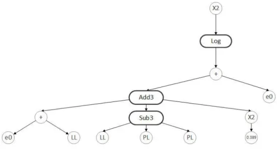
Figure1presents a sample program illustration of evolving GEP, whered1,d2, andd3are the model inputs. Furthermore, the process evolution functions are+,−_,×_,/_{, exponential function (exp()),}

natural logarithm function (ln()), and Inv. The presented model is linear, with coefficientsc0,c1, andc2, while utilizing nonlinear terms [31,32]. For obtainingc0,c1, andc2, a simple least square was applied to the training data. A partial least squares method could also be employed for this objective [18,22]. The important GEP parameters that need to be carefully selected are the tree depth and the quantity of genes. However, minimizing the tree depth generally results in shorter closed-form equations with fewer numbers of terms [29,34].

Infrastructures 2019, 4, x FOR PEER REVIEW 3 of 12

genes. In the GEP framework, the genes in a chromosome may consist of two types of information stored in either the tail or head of genes, i.e., information for generating the overall GEP model and the information from terminals for producing subsequent of the model. Specific details about GEP can be found elsewhere [10,31,32,34,35].

Figure 1 presents a sample program illustration of evolving GEP, where d1, d2, and d3 are the model inputs. Furthermore, the process evolution functions are +, -, ×, /, exponential function (exp()), natural logarithm function (ln()), and Inv. The presented model is linear, with coefficients c0, c1, and

c2, while utilizing nonlinear terms [31,32]. For obtaining c0, c1, and c2, a simple least square was applied to the training data. A partial least squares method could also be employed for this objective [18,22]. The important GEP parameters that need to be carefully selected are the tree depth and the quantity of genes. However, minimizing the tree depth generally results in shorter closed-form equations with fewer numbers of terms [29,34].

Figure 1. Sample gene expression programming (GEP) model.

3. Modeling of Cc for Fine-Grained Soils

3.1. Data Collection

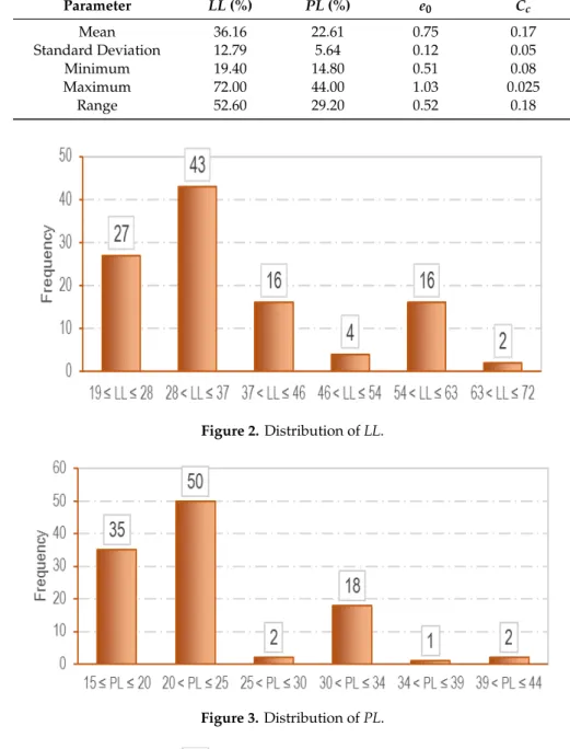
A set of 108 individual consolidation test results obtained from laboratory tests were used to develop the GEP-based prediction equation. As mentioned earlier, the objective of this study was to predict Cc using conventional parameters of fine-grained soils, namely PL, LL, and e0. Here, 101 out of 108 data points corresponded to test results conducted on soil samples collected from different locations in Mashhad, Iran. Soil samples were classified as silty–clayey sand (SC–SM), gravelly lean clay with sand (CL), and silty clay with sand (CL–ML) based on the unified soil classification system. These samples were cored from a depth of 0.5 m to 1.0 m. LL, PL, and e0 were measured for these samples in a laboratory based on ASTM D4318-17 and ASTM D854-14 [36,37]. Furthermore, Cc was measured using an oedometer test based on ASTM D2435-11 [38]. In addition, seven consolidation test results conducted by Malih [39] were integrated into the laboratory database to make it more robust. The descriptive statistics of influential input parameters (i.e., LL, PL, and e0) and the output parameter, i.e., Cc, based on the database utilized for our study is presented in Table 1. Furthermore, Figures 2–5 illustrate the distribution of these parameters using histograms.

Table 1. Descriptive statistics for input and output parameters used in the GEP-based developed model. LL: liquid limit; PL: plastic limit.

Parameter LL (%) PL (%) e0 Cc

Mean 36.16 22.61 0.75 0.17 Standard Deviation 12.79 5.64 0.12 0.05

Figure 1.Sample gene expression programming (GEP) model. 3. Modeling ofCcfor Fine-Grained Soils

3.1. Data Collection

A set of 108 individual consolidation test results obtained from laboratory tests were used to develop the GEP-based prediction equation. As mentioned earlier, the objective of this study was to predictCcusing conventional parameters of fine-grained soils, namelyPL,LL, ande0. Here, 101 out of 108 data points corresponded to test results conducted on soil samples collected from different locations in Mashhad, Iran. Soil samples were classified as silty–clayey sand (SC–SM), gravelly lean clay with sand (CL), and silty clay with sand (CL–ML) based on the unified soil classification system. These samples were cored from a depth of 0.5 m to 1.0 m. LL,PL, ande0were measured for these samples in a laboratory based on ASTM D4318-17 and ASTM D854-14 [36,37]. Furthermore,Ccwas

measured using an oedometer test based on ASTM D2435-11 [38]. In addition, seven consolidation test results conducted by Malih [39] were integrated into the laboratory database to make it more robust. The descriptive statistics of influential input parameters (i.e.,LL,PL, ande0) and the output parameter, i.e.,Cc, based on the database utilized for our study is presented in Table1. Furthermore, Figures2–5

Infrastructures2019,4, 26 4 of 12

Table 1.Descriptive statistics for input and output parameters used in the GEP-based developed model. LL: liquid limit; PL: plastic limit.

Parameter LL(%) PL(%) e0 Cc Mean 36.16 22.61 0.75 0.17 Standard Deviation 12.79 5.64 0.12 0.05 Minimum 19.40 14.80 0.51 0.08 Maximum 72.00 44.00 1.03 0.025 Range 52.60 29.20 0.52 0.18

Infrastructures 2019, 4, x FOR PEER REVIEW 4 of 12

Minimum 19.40 14.80 0.51 0.08 Maximum 72.00 44.00 1.03 0.025 Range 52.60 29.20 0.52 0.18 Figure 2. Distribution of LL. Figure 3. Distribution of PL. Figure 4. Distribution of eo. Figure 2.Distribution ofLL.

Infrastructures 2019, 4, x FOR PEER REVIEW 4 of 12

Minimum 19.40 14.80 0.51 0.08 Maximum 72.00 44.00 1.03 0.025 Range 52.60 29.20 0.52 0.18 Figure 2. Distribution of LL. Figure 3. Distribution of PL. Figure 4. Distribution of eo. Figure 3.Distribution ofPL.

Infrastructures 2019, 4, x FOR PEER REVIEW 4 of 12

Minimum 19.40 14.80 0.51 0.08

Maximum 72.00 44.00 1.03 0.025

Range 52.60 29.20 0.52 0.18

Figure 2. Distribution of LL.

Figure 3. Distribution of PL.

Infrastructures2019,4, 26 5 of 12 Infrastructures 2019, 4, x FOR PEER REVIEW 5 of 12

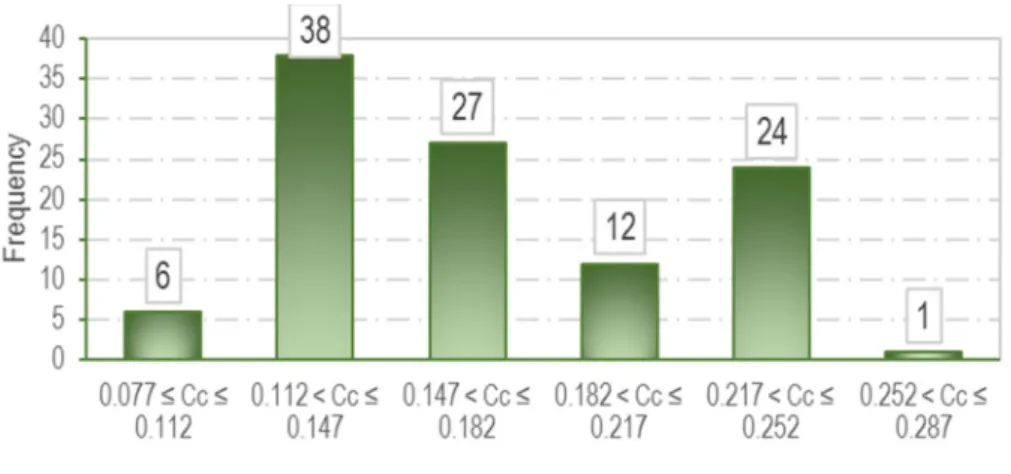
Figure 5. Distribution of Cc.

3.2. Model Structure and Performance

The LL and PL represent the two various states of the soil depending on its water content. The e0 of soil represents the initial ratio of the volume of voids to the solids. Prediction equations for Cc developed by previous studies (see Equation (1)) have clearly indicated that LL, PL, and e0 are the three main parameters that influence Cc [3-9]. Thus, these parameters were considered in the current study to develop a simplified prediction equation for Cc. The main motivation of developing such an equation was that determination of LL, PL, and e0 is straightforward compared to performing any consolidation test that directly determines Cc. Therefore, the developed model is anticipated to result in considerable savings in terms of testing time, technician costs, and laboratory equipment. It should be noted that LL, PL, and e0 are influenced by the natural water content of partially saturated soils, thus making the developed equation applicable to any saturated fine-grained soils [28,39,40]. Mathematically, the developed equation has the following structure:

(

LL

,

PL

,

e

)

f

C

=

showing that Cc is considered to be a function of LL, PL, and e0. In order to develop the GEP-based prediction equation for Cc, a database containing 108 data points was developed. Each data point corresponded to LL, PL, and e0, as well as Cc, for a particular fine-grained soil sample. GeneXproTools 5.0 was used to develop the GEP-based prediction equation in MATLAB [41]. The performances of the developed GEP models were evaluated using the coefficient of determination (R2_{), the root mean squared error (RMSE), and the mean average error (MAE) (21-23), by applying} the following equations:

(

)

(

)

(

)



(

)





−

⋅

−

−

−

=

t

t

h

h

t

t

h

h

R

(

)

n

t

h

RMSE



−

=



−

=

h

t

n

MAE

1

3.2. Model Structure and Performance

TheLLandPLrepresent the two various states of the soil depending on its water content. The e0of soil represents the initial ratio of the volume of voids to the solids. Prediction equations forCc

developed by previous studies (see Equation (1)) have clearly indicated thatLL,PL, ande0are the three main parameters that influenceCc[3–9]. Thus, these parameters were considered in the current

study to develop a simplified prediction equation forCc. The main motivation of developing such

an equation was that determination ofLL,PL, ande0 is straightforward compared to performing any consolidation test that directly determinesCc. Therefore, the developed model is anticipated to

result in considerable savings in terms of testing time, technician costs, and laboratory equipment. It should be noted thatLL,PL, ande0are influenced by the natural water content of partially saturated soils, thus making the developed equation applicable to any saturated fine-grained soils [28,39,40]. Mathematically, the developed equation has the following structure:

Cc= f(LL,PL,e0), (1)

showing thatCcis considered to be a function ofLL,PL, ande0. In order to develop the GEP-based

prediction equation forCc, a database containing 108 data points was developed. Each data point

corresponded toLL,PL, ande0, as well asCc, for a particular fine-grained soil sample. GeneXproTools

5.0 was used to develop the GEP-based prediction equation in MATLAB [41]. The performances of the developed GEP models were evaluated using the coefficient of determination (R2), the root mean squared error (RMSE), and the mean average error (MAE) (21-23), by applying the following equations:

R2= Pn i=1 hi−hi ti−ti q Pn i=1 hi−hi 2 ·Pn i=1 ti−ti 2 , (2) RMSE= s Pn i=1(hi−ti) 2 n , (3) MAE= 1 n n X i=1 |_hi−_ti|_{. (4)}

In these equations,hiandtiare measured and predicted output (Cc) values, respectively, for the ith data point. Furthermore,hiandtiare averages of the measured and predicted values, respectively,

Infrastructures2019,4, 26 6 of 12

3.3. Model Development

The database was divided into two subsets in order to avoid an overfitting issue, a training subset and a validation subset. The GEP-based model was trained using the training subset, while the validation subset was used for validating purposes and for avoiding overfitting [34]. The final model (prediction equation) was selected based on model simplicity and the performances of the training and validation subsets. Performance criteria were based on the highestR2_{and lowestRMSEandMAEof} the training and validation subsets. After training, the candidate models were applied to the unseen validation subset to ensure their good performance. The proportion of training to validation subset sizes with respect to the whole data is commonly selected as 60%–75% and 25%–40%, respectively. In the current study, 75% (81 data points) and 25% (27 data points) of total data points were assigned to the training subset and validation subset, respectively.

The GEP algorithm was executed several times with a varied combination of influential parameters in order to identify the best model. This process was based on values suggested by previous works [31,32,34]. Table2includes the parameters of various runs. Reasonably large numbers were considered for size of population and generations to guarantee that optimal models were achieved. In the developed GEP-based model, individuals were identified and transferred into further generations based on a fitness evaluation carried out with roulette wheel sampling, considering elitism. Such an evaluation could guarantee successful cloning of the best individual. Furthermore, variations in the population were carried out through genetic operators on the chosen chromosomes, including crossover, mutation, and rotation [10].

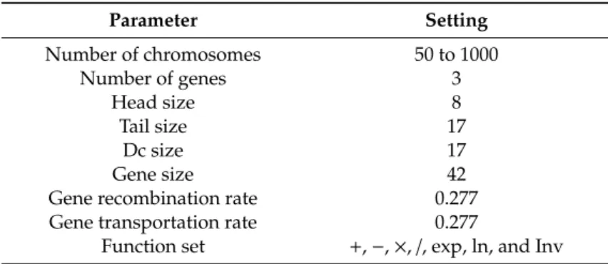
Table 2.Parameters used for implementation of the GEP-based model.

Parameter Setting Number of chromosomes 50 to 1000 Number of genes 3 Head size 8 Tail size 17 Dc size 17 Gene size 42

Gene recombination rate 0.277 Gene transportation rate 0.277

Function set +,−_,×_,/_{, exp, ln, and Inv}

In every GEP-based model, the values of the setting parameters have a significant impact on model performance. These parameters include the quantity of genes and chromosomes, in addition to a gene’s head size and the rate of genetic operators. Since minor information was available about GEP parameters in the literature, appropriate settings were selected based on a trial and error scheme (see Table2).

Furthermore, to facilitate the development of the GEP-based model, the following closed-form equation was developed and utilized:

Cc=e0+ " e0+2LL e0−6.87 # ×h−_0.35+LL2i_{+ [log(2e0+2LL}−_2PL+0.15)]2_{. (5)}

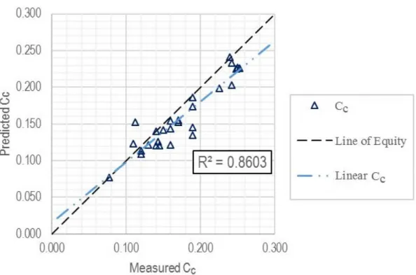
Figures6–8present the measured values ofCcobtained from laboratory experiments versus

predicted values. These figures represent the measured values versus predicted values for the training subset, validation subset, and entire set, respectively. Furthermore, Table3summarizes the GEP-based model performance in terms ofR2,RMSE, andMAEfor these sets. Smith [42] has stated that for a coefficient of determination of|R|>0.8, a strong correlation exists between measured and predicted values. Based on Table3, the developed GEP-based model had a highR2_{for the training subset,}

Infrastructures2019,4, 26 7 of 12

validation subset, and entire dataset. In addition, the model exhibited a relatively lowRMSEandMAE for all of these sets.

Infrastructures 2019, 4, x FOR PEER REVIEW 7 of 12

that for a coefficient of determination of |R|> 0.8, a strong correlation exists between measured and predicted values. Based on Table 3, the developed GEP-based model had a high R2 _{for the training}

subset, validation subset, and entire dataset. In addition, the model exhibited a relatively low RMSE

and MAE for all of these sets.

Figure 6. Predicted versus measured Cc for the training subset.

Figure 7. Predicted versus measured Cc for the validation subset.

Figure 6.Predicted versus measuredCcfor the training subset.

Infrastructures 2019, 4, x FOR PEER REVIEW 7 of 12

that for a coefficient of determination of |R|> 0.8, a strong correlation exists between measured and

predicted values. Based on Table 3, the developed GEP-based model had a high R2 _{for the training}

subset, validation subset, and entire dataset. In addition, the model exhibited a relatively low RMSE

and MAE for all of these sets.

Figure 6. Predicted versus measured Cc for the training subset.

Figure 7. Predicted versus measured Cc for the validation subset.

Infrastructures2019,4, 26 8 of 12

Infrastructures 2019, 4, x FOR PEER REVIEW 8 of 12

Figure 8. Predicted versus measured Ccfor the entire dataset (training + validation).

Table 3. Model performance. RMSE: root mean squared error; MAE: mean average error.

Set Number of

Data Points R2 RMSE MAE

Training subset 81 0.8231 0.0269 0.0213

Validation subset 27 0.8603 0.0237 0.0189

Entire dataset 108 0.8320 0.0262 0.0207

3.4. Additional evaluation of model performance

In this section, the performance of the developed GEP-based model is evaluated based on various statistical parameters found in the literature. These statistical parameters, along with their acceptance criteria, are presented in Table 4. The parameters used in this table are all as previously defined. Furthermore, the developed model was evaluated based on these statistical parameters, and the results are presented in this table. As can be seen in Table 4, the developed model met all of the criteria for additional statistical parameters, revealing the decent performance of the proposed model.

Table 4. Evaluating the developed GEP-based model using additional statistical parameters.

Statistical Parameter Source Criteria

Evaluation for GEP-Based Model

(

)

h

t

h

k

=



×

(

)

'

t

t

h

k

=



×

(

)

2

1

R

Ro

R

R

=

×

−

−

Figure 8.Predicted versus measuredCcfor the entire dataset (training+validation). Table 3.Model performance. RMSE: root mean squared error; MAE: mean average error.

Set Number of Data Points R 2 _{RMSE MAE} Training subset 81 0.8231 0.0269 0.0213 Validation subset 27 0.8603 0.0237 0.0189 Entire dataset 108 0.8320 0.0262 0.0207

3.4. Additional Evaluation of Model Performance

In this section, the performance of the developed GEP-based model is evaluated based on various statistical parameters found in the literature. These statistical parameters, along with their acceptance criteria, are presented in Table4. The parameters used in this table are all as previously defined. Furthermore, the developed model was evaluated based on these statistical parameters, and the results are presented in this table. As can be seen in Table4, the developed model met all of the criteria for additional statistical parameters, revealing the decent performance of the proposed model.

Table 4.Evaluating the developed GEP-based model using additional statistical parameters.

Statistical Parameter Source Criteria Evaluation for

GEP-Based Model k= Pn i=1(hi×ti) h2 i

Golbraikh and Tropsha [43] 0.85<k<1.15 1.001

k0= Pn

i=1(hi×ti)

t2

i

Roy and Roy [44] 0.85<k’<1.15 0.989

Rm=R2×

1−

√

R2−_Ro2

Roy and Roy [44] 0.5<Rm 0.503

Ro2=1− Pn i=1(ti−hoi) 2 Pn i=1(ti−ti)

2,ho_i =k×ti Roy and Roy [44] Should be close to 1.0 1.000

Ro02₌₁− Pn i=1(ti−toi) 2 Pn i=1 hi−hi

2 Roy and Roy [44] Should be close to 1.0 0.998

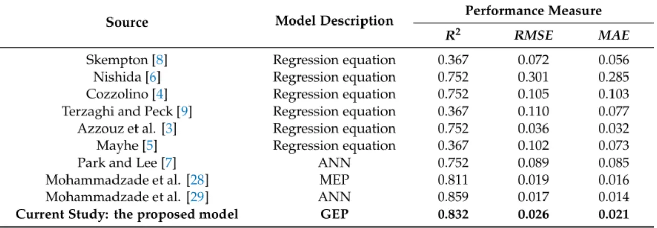
Table5presents a comparison of the developed GEP-based model to previous models found in the literature. The previous models consist of either regression-based equations or robust AI methods,

Infrastructures2019,4, 26 9 of 12

such as MEP, ANNs, or MGGP. It is worth mentioning that these AI methods do not provide any closed-form solution. The AI methods had a relatively highR2, mainly due to their black-box nature of connecting inputs and outputs. Nevertheless, the developed GEP-based model had a higherR2 compared to the existing AI methods. However, MEP, ANNs, and MGGP had a lower error in terms of RMSEandMAE.

Table 5.Performance comparison of the current developed GEP-based model to existing models. MEP: multi-expression programming; ANN: artificial neural network.

Source Model Description Performance Measure

R2 RMSE MAE

Skempton [8] Regression equation 0.367 0.072 0.056 Nishida [6] Regression equation 0.752 0.301 0.285 Cozzolino [4] Regression equation 0.752 0.105 0.103 Terzaghi and Peck [9] Regression equation 0.367 0.110 0.077 Azzouz et al. [3] Regression equation 0.752 0.036 0.032 Mayhe [5] Regression equation 0.367 0.102 0.073

Park and Lee [7] ANN 0.752 0.089 0.085

Mohammadzade et al. [28] MEP 0.811 0.019 0.016 Mohammadzade et al. [29] ANN 0.859 0.017 0.014

Current Study: the proposed model GEP 0.832 0.026 0.021

Based on Table5, the developed GEP-based model outperformed the regression models, since the regression models considered only a small quantity of base functions. Therefore, such models could not be used for the complex interactions of soil parameters (i.e.,LL,PL, ande0) andCc. However, the

developed GEP-based model considered a variety of base functions and their combination in order to achieve a closed-form equation with high performance. The developed GEP-based model directly considered the experimental data with no prior assumptions. In other words, contrary to traditional regression models, GEP did not assume any predefined shape for the solution equation. The high values ofR2_{presented in Table5indicate that the developed GEP-based model was very successful at} fitting the measuredCcto the input parameters ofLL,PL, ande0.

4. Conclusions

Ccis a significant parameter in determining the settlement of fine-grained soil layers subjected

to loads, such as in buildings, vehicles, and infrastructure. IfCcis not estimated accurately, soil

settlement is not predicted accurately. Thus, determiningCcis of significant importance in settlement

calculations. However, measuringCcusing the traditional oedometer test method is time-consuming,

needs skilled technicians, and requires special laboratory equipment. Therefore, the estimation ofCc

using other parameters of fine-grained soils, such asLL,PL, ande0, would eliminate the time and costliness associated with the oedometer test. In this study, GEP was employed to develop a model for estimatingCcusingLL,PL, ande0. Here, 108 data points containingCc,LL,PL, ande0were used to

train and validate the model. The model was developed based on tuned calibration parameters using trial and error. A closed-form solution was derived from the developed GEP-based model, which is anticipated to aid geotechnical researchers in determiningCcwith considerable savings in associated

time and costs. This closed-form equation for predictingCcwas employed to develop surface charts to

predictCcbased onLLandPLfor a certaine0.

The performance of the developed GEP-based model was evaluated using the coefficient of determination (R2_{) and two error measures, namely root mean squared error (RMSE) and mean average} error (MAE). TheR2values were 0.8231, 0.8603, and 0.8320 for the training subset, validation subset, and entire dataset, respectively. In addition,RMSEwas 0.0269, 0.0237, and 0.0262 for the training subset, validation subset, and entire dataset, respectively. A highR2 and low error indicated the highly acceptable performance of the GEP-based model. Additional performance measures found

Infrastructures2019,4, 26 10 of 12

in the literature were employed to further evaluate the performance of the developed GEP-based model. This evaluation revealed that the model had a decent performance based on additional performance measures.

Contrary to the classical models for estimatingCc, such as regression models, the developed

GEP-based model revealed highly nonlinear behavior and included a complex combination of influential input parameters (i.e.,LL,PL, ande0). In general,Ccwas positively correlated withe0. Furthermore,LL ande0had a higher influence on the estimation ofCccompared toPL. A comparison of the developed

model to previous models in the literature revealed its good performance, which guarantees the use of this GEP-based model in practical applications.

Author Contributions:Review, formal analysis, methodology, modeling data curation and analyzing the results, D.M.S., A.M., and S.-F.K.; soil expertise, D.M.S., J.H.M.T., S.-F.K., and E.N.; machine learning expertise, A.M. and D.M.S.; management, conceptualization, writing, and administration A.M.; data visualization, data handling, support and data assistant; E.N.; supervision, resources, software, expertise, revision, validation and verifying the results, J.H.M.T.

Funding:This research received no externa funding.

Conflicts of Interest:The authors declare no conflicts of interest. References

1. Tiwari, B.; Ajmera, B. New correlation equations for compression index of remolded clays. J. Geotech. Geoenviron. Eng.2011,138, 757–762. [CrossRef]

2. Carter, M.; Bentley, S.P.Correlations of Soil Properties; Pentech Press Publishers: Philadelphia, NJ, USA, 1991. 3. Azzouz, A.S.; Krizek, R.J.; Corotis, R.B. Regression analysis of soil compressibility.SOILS Found.1976,16,

19–29. [CrossRef]

4. Cozzolino, V. Statistical forecasting of compression index. In Proceedings of the Fifth International Conference on Soil Mechanics and Foundation Engineering, Paris, France, 17–22 July 1961; pp. 51–53.

5. Mayhe, P. Cam-clays predictions of undrained strength.J. Geotech. Geoenviron. Eng. 1980,106, 1219–1242. 6. Nishida, Y. A brief note on compression index of soil.J. Soil Mech. Found. Div.1956,82, 1–14.

7. Park, H.I.; Lee, S.R. Evaluation of the compression index of soils using an artificial neural network.Comput. Geotech.2011,38, 472–481. [CrossRef]

8. Skempton, A.W.; Jones, O.T.; Quennell, A.M. Notes on the compressibility of clays.Q. J. Geol. Soc.1944,100, 119–135. [CrossRef]

9. Terzaghi, K.; Peck, R.B.; Mesri, G.Soil Mechanics in Engineering Practice; John Wiley & Sons: Dallas, TX, USA, 1996.

10. Alavi, A.H.; Gandomi, A.H. A robust data mining approach for formulation of geotechnical engineering systems.Eng. Comput.2011,28, 242–274. [CrossRef]

11. Choubin, B.; Moradi, E.; Golshan, M.; Adamowski, J.; Sajedi-Hosseini, F.; Mosavi, A. An ensemble prediction of flood susceptibility using multivariate discriminant analysis, classification and regression trees, and support vector machines.Sci. Total. Environ.2019,651, 2087–2096. [CrossRef]

12. Rezakazemi, M.; Mosavi, A.; Shirazian, S. ANFIS pattern for molecular membranes separation optimization. J. Mol. Liq.2019,274, 470–476. [CrossRef]

13. Mosavi, A.; Ozturk, P.; Chau, K.-W. Flood Prediction Using Machine Learning Models: Literature Review. Water2018,10, 1536. [CrossRef]

14. Mosavi, A.; Lopez, A.; Varkonyi-Koczy, A.R. Industrial applications of big data: State of the art survey. In Proceedings of the International Conference on Global Research and Education, Lasi, Romania, 25–28 September 2017; pp. 225–232.

15. Mosavi, A.; Bathla, Y.; Varkonyi-Koczy, A. Predicting the future using web knowledge: State of the art survey. In Proceedings of the International Conference on Global Research and Education, Lasi, Romania, 25–28 September 2017; pp. 341–349.

Infrastructures2019,4, 26 11 of 12

17. Mosavi, A.; Rabczuk, T. Learning and intelligent optimization for material design innovation. In Proceedings of the International Conference on Learning and Intelligent Optimization, Russia, Novgorod, 19 June 2017; pp. 358–363.

18. Mosavi, A.; Rabczuk, T.; Varkonyi-Koczy, A.R. Reviewing the novel machine learning tools for materials design. In Proceedings of the International Conference on Global Research and Education, Lasi, Romania, 23 September 2017; pp. 50–58.

19. Mosavi, A.; Varkonyi-Koczy, A.R. Integration of machine learning and optimization for robot learning. In Recent Global Research and Education: Technological Challenges; Springer: Lasi, Romaria, 2017; pp. 349–355. 20. Mosavi, A.; Edalatifar, M. A Hybrid Neuro-Fuzzy Algorithm for Prediction of Reference Evapotranspiration.

In Proceedings of the International Conference on Global Research and Education, Kaunas, Lithuania, 4 September 2017; pp. 235–243.

21. Torabi, M.; Mosavi, A.; Ozturk, P.; Varkonyi-Koczy, A.; Istvan, V. A hybrid machine learning approach for daily prediction of solar radiation. In Proceedings of the International Conference on Global Research and Education, Kaunas, Lithuania, 24–27 September 2018; pp. 266–274.

22. Das, S.K.; Basudhar, P.K. Prediction of residual friction angle of clays using artificial neural network.Eng. Geol.2008,100, 142–145. [CrossRef]

23. Das, S.K.; Biswal, R.K.; Sivakugan, N.; Das, B. Classification of slopes and prediction of factor of safety using differential evolution neural networks.Environ. Earth Sci.2011,64, 201–210. [CrossRef]

24. Daryaei, M.; Kashefipour, S.M.; Ahadian, J.; Ghobadian, R. Modeling the compression index of fine soils using artificial neural network and comparison with the other empirical equations. J. Water Soil2010,5, 312–333.

25. Farkhonde, S.; Bolouri, J. Estimation of compression index of clayey soils using artificial neural network. In Proceedings of the Fifth National Conference on Civil Engineering, Mashhad, Iran, 10 May 2018.

26. Kumar, V.P.; Rani, C.S. Prediction of compression index of soils using artificial neural networks (ANNs).Int. J. Eng. Res. Appl.2011,1, 1554–1558.

27. Talaei-Khoei, A.; Wilson, J.M.; Kazemi, S.-F. Period of Measurement in Time-Series Predictions of Disease Counts from 2007 to 2017 in Northern Nevada: Analytics Experiment.JMIR Public Health Surveill.2019,5, e11357. [CrossRef] [PubMed]

28. Mohammadzadeh, D.; Bazaz, J.B.; Yazd, S.V.J.; Alavi, A.H. Deriving an intelligent model for soil compression index utilizing multi-gene genetic programming.Environ. Earth Sci.2016,75, 262. [CrossRef]

29. Mohammadzadeh, D.; Bazaz, J.B.; Alavi, A.H. An evolutionary computational approach for formulation of compression index of fine-grained soils.Eng. Appl. Artif. Intell.2014,33, 58–68. [CrossRef]

30. Kazemi, S.F.; Shafahi, Y. An Integrated Model Of Parallel Processing And PSO Algorithm For Solving Optimum Highway Alignment Problem. In Proceedings of the ECMS, Aesund, Norway, 12 June 2013; pp. 551–557.

31. Ferreira, C.Gene Expression Programming: Mathematical Modeling by an Artificial Intelligence; Springer: Bristol, UK, 2006; Volume 21.

32. Ferreira, C. Gene expression programming and the evolution of computer programs. InRecent Developments in Biologically Inspired Computing; Springer: Oxford, UK, 2004; pp. 82–103.

33. Koza, J.R.Genetic Programming: on the Programming of Computers by Means of Natural Selection; MIT Press: London, UK, 1992; Volume 1.

34. Ferreira, C. Gene expression programming in problem solving. InSoft Computing and Industry; Springer: Angra do Heroismo, Portugal, 2002; pp. 635–653.

35. Batioja-Alvarez, D.D.; Kazemi, S.-F.; Hajj, E.Y.; Siddharthan, R.V.; Hand, A.J.T. Probabilistic Mechanistic-Based Pavement Damage Costs for Multitrip Overweight Vehicles. J. Transp. Eng. Part B Pavements2018,144, 04018004. [CrossRef]

36. Standard Test Methods for Liquid Limit, Plastic Limit, and Plasticity Index of Soils; ASTM International: Washington, DC, USA, 2017.

37. ASTM.Standard Test Method for Bulk Specific Gravity and Density of Non-Absorptive Compacted Asphalt Mixtures; ASTM International: Washington, DC, USA, 2017.

38. Standard Test Methods for One-Dimensional Consolidation Properties of Soils Using Incremental Loading; ASTM International: Washington, DC, USA, 2011.

Infrastructures2019,4, 26 12 of 12

39. Gandomi, A.H.; Mohammadzadeh, D.; Pérez-Ordóñez, J.L.; Alavi, A.H. Linear genetic programming for shear strength prediction of reinforced concrete beams without stirrups.Appl. Soft Comput.2014,19, 112–120. [CrossRef]

40. Ziaee, S.A.; Sadrossadat, E.; Alavi, A.H.; Shadmehri, D.M. Explicit formulation of bearing capacity of shallow foundations on rock masses using artificial neural networks: Application and supplementary studies. Environ. Earth Sci.2015,73, 3417–3431. [CrossRef]

41. Gepsoft GeneXproTools, version 5.0; Gepsoft: Bristol, UK, 2014.

42. Smith, G.N.Probability and Statistics in Civil Engineering; Collins Professional and Technical Books; Collins: London, UK, 1986; 244p.

43. Golbraikh, A.; Tropsha, A. Beware of q2!J. Mol. Graph. Model.2002,20, 269–276. [CrossRef]

44. Roy, P.P.; Roy, K. On Some Aspects of Variable Selection for Partial Least Squares Regression Models.QSAR Comb. Sci.2008,27, 302–313. [CrossRef]

©2019 by the authors. Licensee MDPI, Basel, Switzerland. This article is an open access article distributed under the terms and conditions of the Creative Commons Attribution (CC BY) license (http://creativecommons.org/licenses/by/4.0/).