Reinforcement learning from internal, partially
correct, and multiple demonstrations
Mao Li
Doctor of Philosophy
University of York
Computer Science
Abstract
Typically, a reinforcement learning agent interacts with the environment and learns how to select an action to gain cumulative reward in one trajectory of a task. However, classic rein-forcement learning emphasises knowledge free learning processes. The agent only learns from state-action-reward-next state samples. The learning process has the problem of sample ineffi-ciency and needs a huge number of interactions to converge upon an optimal policy. One of the solutions to deal with this challenge is to employ human behaviour records in the same task as demonstrations for the agent to speed up the learning process.
Demonstrations are not, however, from the optimal policy and may be in conflict in many states especially when demonstrations come from multiple resources. Meanwhile, the agent’s behaviour in the learning process can be used as demonstration data. To address the research gaps mentioned above, three novel techniques, including; introspective reinforcement learning, two-level Q-learning, and the radius restrained weighted vote, are proposed in this thesis. Introspective reinforcement learning uses a priority queue as a filter to select qualified agent behaviours during the learning process as demonstrations. It applies reward shaping to give the agent an extra reward when it performs similar behaviours as demonstrations in the filter. The two-level-Q-learning deals with the issue of conflicting demonstrations. Two Q-tables (or Q-net in function approximation) for storing state-expert value and state-action value are proposed respectively. The two-level-Q-learning allows the agent not only to learn a strategy from selected actions but also to learn to distribute credits to experts through trial and error. The Radius restrained weighted vote can derive a guidance policy from demonstrations which satisfy a restriction through a hyper-parameter radius. The Radius restrained weighted vote applied the Gaussian distances between the current state and demonstrations as weights of the votes. Softmax was applied to the total number of weighted votes from all candidate demonstrations to derive the guidance policy.
Acknowledgements
First of all, I would like to thank my supervisor Dr. Daniel Kudenko, who guided me to the field of reinforcement learning and showed me what a good researcher is. I really appreciate his contribution of time and ideas to make my Ph.D. experience so valuable and stimulating. He continuously gave me patient guidance and support. His rigorousness and enthusiasm for research were so motivating for me. I am also thankful to Dr.James Cussens, my internal auditor, who helped me to review every milestone of my Ph.D. and who provided constructive suggestions on my thesis. My sincere gratitude is also given to Prof. Ann Nowé, who spent her time reading my thesis and attend my thesis viva.
My wife, Dr.Wei Zheng, gave me meticulous care in daily life and spiritual encouragement. Her love, understanding and encouragement supported me along this journey. My parents, my first teachers, have contributed immensely to my personal development; they have encouraged me to explore science and engineering since I was very young. I thank my family for their love and support. This thesis is dedicated to them.
My sincere gratitude also goes to my friends in and outside York, who cheered me up and encouraged me to move forward.
Finally, thanks Dr.Bertie Dockerill for proofreading the thesis.Thanks also to those who con-tributed to online-course projects. Without the equal right of education by internet, I could not share the opportunity to learn such good training courses and explore more in my research field.
Thank you!
Declaration
I declare that this thesis is a presentation of original work and I am the sole author. This work has not previously been presented for an award at this, or any other, University. All sources are acknowledged as References.
Some of the material contained in this thesis has appeared in the following published or awaiting publication papers:
1. Li, M., Brys, T., Kudenko, D. (2018). Introspective reinforcement learning and learning from demonstration. In Proceedings of the 17th International Conference on Autonomous Agents and MultiAgent Systems, (pp. 19921994).
2. Li, M., Kudenko, D. (2018). Reinforcement learning from multiple experts demonstra-tions. In Workshop on Adaptive Learning Agents (ALA) at the Federated AI Meeting, volume 18.
3. Li, M., Brys, T., Kudenko, D. Introspective Q-learning and learning from demonstration. The Knowledge Engineering Review. 2019.
4. Li, M., Yi, W., Kudenko, D. Two-level Q-learning: learning from conflict demonstrations. The Knowledge Engineering Review. 2019.
Contents
Abstract i
Acknowledgements iii
1 Introduction 1
1.1 General approaches to AI from RL . . . 1
1.2 Research Gap . . . 3
1.2.1 Delayed feedback and credit allocation . . . 3
1.2.2 Representation of state space . . . 4
1.2.3 Explore and exploit the balance . . . 5
1.2.4 Sample inefficiency . . . 5 1.2.5 Sparse Rewards . . . 6 1.3 Research Motivation . . . 6 1.4 Hypotheses . . . 7 1.5 Contribution . . . 8 1.5.1 Introspective Q-learning . . . 8
1.5.2 RL from conflicting demonstrations . . . 9
1.5.3 RL from massive and imbalanced demonstrations . . . 9 ix
x CONTENTS
1.6 Structure of the Thesis . . . 10
1.7 Chapter Summary . . . 12
2 Reinforcement Learning Background 13 2.1 Overview . . . 13
2.2 The Markov Process . . . 14
2.2.1 Markov Chains . . . 14
2.2.2 The Markov Reward Process . . . 15
2.2.3 The Markov Decision Process . . . 15
2.3 Model-based policy estimation . . . 16
2.4 Model-free policy estimation . . . 17
2.4.1 The Monte Carlo estimation . . . 17
2.4.2 Temporal difference estimation . . . 18
2.5 Policy improvement . . . 19
2.5.1 Generalised policy improvement . . . 19
2.5.2 TD-learning . . . 21
2.6 Function approximation . . . 23
2.6.1 Deep Reinforcement learning . . . 25
2.6.2 Improvement of DQN . . . 27
2.7 Policy gradient . . . 30
2.7.1 REINFORCE . . . 30
2.7.2 Reducing the variance of the gradient . . . 31
CONTENTS xi
2.7.4 Off-policy gradient descent . . . 33
2.7.5 DPG and DDPG . . . 35
2.8 Summary . . . 35
3 Reinforcement Learning with External Information 37 3.1 Key challenges . . . 37
3.2 Sources of Information for RL . . . 38
3.2.1 Heuristic rules . . . 38
3.2.2 Online Advice . . . 39
3.2.3 Policy transfer from similar tasks . . . 39
3.2.4 RL from Demonstrations . . . 40
3.3 Injection of information into RL . . . 41
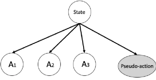
3.3.1 Reward shaping . . . 42 3.3.2 Pseudo-action . . . 44 3.3.3 Probabilistic reuse . . . 45 3.3.4 Pre-training . . . 45 3.4 Imitation learning . . . 46 3.4.1 Behavioural cloning . . . 46 3.4.2 Interactive demonstrator . . . 47
3.4.3 Inverse reinforcement learning . . . 48
3.5 Research gaps . . . 48
xii CONTENTS
4 Introspective Reinforcement learning 52
4.1 Research Motivation . . . 52
4.2 Assumption . . . 53
4.3 Methodology of Introspective RL . . . 54
4.3.1 Collecting the experiences . . . 55
4.3.2 Defining the Potential Function . . . 56
4.3.3 Pulling it together . . . 58
4.4 Speed up from demonstrations . . . 59
4.5 Experimental validation . . . 60
4.5.1 CartPole . . . 60
4.5.2 Complex domain application: Super Mario . . . 63
4.6 Summary . . . 66
5 Q-learning from multiple conflict demonstration 69 5.1 Conflicting demonstrations . . . 69
5.2 Learn value of experts . . . 70
5.3 Multiple domain knowledge sources . . . 70
5.4 Two-level structure of reinforcement learning . . . 71
5.5 Synchronised Q-table updating . . . 72
5.6 Pulling it all together . . . 72
5.7 Empirical Study . . . 72
5.8 Maze navigation . . . 74
CONTENTS xiii
5.10 Application in complex domain . . . 81
5.11 Pong . . . 81
5.12 Summary . . . 81
6 Q-learning from a massive number of imbalanced demonstrations 85 6.1 Related research . . . 86
6.2 Radius restrained weighted voting . . . 88
6.2.1 Restrain radius . . . 88 6.2.2 Weighted voting . . . 89 6.2.3 Algorithm . . . 90 6.3 Case study . . . 90 6.4 Experiments . . . 92 6.4.1 Maze domain . . . 92
6.4.2 Flappy bird domain . . . 95
6.5 Summary . . . 97
7 Conclusion 99 7.1 Contributions . . . 99
7.2 Introspective RL . . . 100
7.3 RL from conflict demonstrations . . . 101
7.4 RL from massive demonstrations . . . 102
7.5 Limitations . . . 103
7.6 Combination . . . 103
Bibliography 104
List of Tables
6.1 Table to compare deriving policy from demonstrations . . . 91
List of Figures
1.1 Agent environment interaction . . . 3
1.2 Thesis structure . . . 11
2.1 Tile coding (Sutton et al., 1998) . . . 25
2.2 A popular single stream Q-network (top) and the dueling Q-network (bottom) (Wang et al., 2015) . . . 28
2.3 Actor-Critic learning process . . . 33
3.1 Sparse reward MDP . . . 42
3.2 Sparse reward MDP . . . 43
3.3 A pseudo action with real actions . . . 44
4.1 5 states MDP . . . 53
4.2 Cartpole domain is an inverted Pendulum (Michie and Chambers, 1968) . . . 61
4.3 CartPole learning curves of Q(λ)-learning and Introspective RL without any external demonstrations. Learning rateα = 016.25, discount rate γ = 1.0,λ= 0.25 and an ϵ-greedy exploration strategy withϵ = 0.05. Tile coding was used as the function approximation with 16 10×10 tilings. . . 62
xviii LIST OF FIGURES
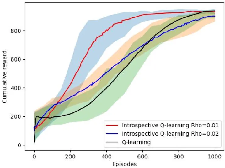
4.4 CartPole learning curves of Q(λ)-learning, and Introspective RL for differentλ. Learning rate α = 016.25, discount rate γ = 1.0, λ = 0.25 and an ϵ-greedy explo-ration strategy withϵ= 0.05. Tile coding was used as the function approximation with 1610×10tilings. . . 63 4.5 CartPole learning curves of Q(λ)-learning, RL from Demonstration, and
Intro-spective RL with demonstration from a human player with a performance score between 400 to 650. Learning rate α = 016.25, discount rate γ = 1.0, λ = 0.25 and an ϵ-greedy exploration strategy withϵ = 0.05. Tile coding was used as the function approximation with 16 10×10 tilings. . . 64 4.6 Screen shot of Super Mario benchmark (Karakovskiy and Togelius, 2012) . . . . 65 4.7 Super Mario Domain learning curves of Q(λ)-learning, and Introspective RL
without demonstration. Learning rate α = 0.001, discount factor γ = 0.9, ϵ -greedy exploration with ϵ= 0.05 ,λ = 0.5 with an additional σ = 0.5 . . . 66 4.8 Super Mario Domain learning curves of Q(λ)-learning, RLfD, and Introspective
RL with 20 demonstration episodes from a human player with a performance score between 400 to 650. Learning rate α = 0.001, discount factor γ = 0.9,
ϵ-greedy exploration with ϵ= 0.05 ,λ = 0.5 with an additional σ= 0.5 . . . 67
5.1 The structure of 2-level Q-learning, including two Q-tables: a high-level Q-table and low-level Q-table . . . 71 5.2 Maze divided into three non-overlapping regions . . . 74 5.3 Performance comparison of TLQL, Q-learning and CHAT (Wang and Taylor,
2017) in the domain of maze navigation. Learning rate α = 0.01, discount rate
γ = 0.99,ϵ-greedy ϵ= 0.1. . . 76 5.4 Comparison Q-learning of TLQL with 1 expert, 2 experts and 3 experts.
Learn-ing rate α= 0.01, discount rate γ = 0.99,ϵ-greedy ϵ= 0.1. . . 76 5.5 Coloured flags visiting problem domain . . . 77 5.6 Three correct examples sequence of visiting flags . . . 78
5.7 Three demonstrators and their view of the environment . . . 79
5.8 Performance comparison of TLQL,CHAT (Wang and Taylor, 2017) and Q-learning in the domain of coloured flags visiting. Learning rate α = 0.01, discount rate γ = 0.99,ϵ-greedy ϵ= 0.1. . . 80
5.9 Comparison of TLQL with different number of experts and regular Q-learning in the domain of coloured flags visiting. Learning rate α = 0.01, discount rate γ = 0.99,ϵ-greedy ϵ= 0.1. . . 80
5.10 Pong: A game of Atari 2660 . . . 82
5.11 Structure of neural network of DQN and expert . . . 82
5.12 Comparison of TLQL with CHAT (Wang and Taylor, 2017) and regular Q-learning in the domain of Atari game Pong. . . 83
6.1 3x3 grid domain with one correction demonstration . . . 87
6.2 Initialised Q-value 3x3 grid domain via SBS (Brys et al., 2015) . . . 88
6.3 Initialised Q-value 3x3 grid domain . . . 89
6.4 Compare RRWV, SBS and kNN Transfer . . . 92
6.5 Maze domain with demonstration . . . 93
6.6 Derive a policy from demonstration in 9x10 maze via SBS . . . 93
6.7 Derive a policy from the demonstration in 9x10 maze via RRWV radius=1 and 2 94 6.8 Compare the RRWV and SBS . . . 94
6.9 Domain of flappy bird game . . . 95
6.10 Neural network structure used in Flappy bird game . . . 96
6.11 preprocessing state of flappy bird . . . 96
6.12 Compare RRWV, SBS and DQN in Flappy bird game . . . 97
Chapter 1
Introduction
In this chapter, an overview of the thesis is given. It includes a definition of reinforcement learning (RL), the motivation for the research, identification of a research gap and my contri-bution to addressing this. This chapter also includes an outline of the structure of the rest of the thesis.
1.1
General approaches to AI from RL
One definition of artificial intelligence (AI) is that it is an agent that is able to observe the environment and execute actions to maximise its chance of approaching its goals successfully (Russell and Norvig, 2016; Poole et al., 1998; Nilsson, 1998). Turing, the creator of modern computing opined, in a 1950 paper, that, "instead of trying to produce a programme to simulate the adult mind, why not rather try to produce one which simulates the child’s? If this were then subjected to an appropriate course of education one would obtain the adult brain" (Turing, 1950).
Machine learning(ML) constructs a mathematical model based on training data, in order to make predictions or decisions without being explicitly programmed to perform the task. Per-formance of an ML algorithm is improved using experiences with the training time (Friedman
2 Chapter 1. Introduction
et al., 2001). Machine learning has been divided into three categories: supervised learning, un-supervised learning, and reinforcement learning. Supervised learning uses algorithms to train an agent to learn the mapping from a feature space to a target space through a labelled dataset (Mohri et al., 2018, chapter 2). Unsupervised learning agents have been trained on datasets without labels. Unsupervised learning is generally used, as Ghahramani (2003) notes, to dis-cover hidden patterns or groupings in a dataset. In contrast, reinforcement learning (RL) is the paradigm which addresses sequential decision making in a task. Unlike supervised learning, the goal of reinforcement learning is to find the optimal decision sequence to maximise the cumulative utilities of the agent (Barto, 1997).
To achieve the goal of creating an intelligence agent, AI researchers draw lessons from psy-chologists and biologist to educate agents through giving them reward and punishment signals. Skinner (1990) considers reinforcement to be the key to learning. The main principle of RL is giving positive reinforcement and negative reinforcement signals to an agent based on all of its actions. As the name implies, positive reinforcement gives a reward signal to the agent. For instance, training a mouse to touch a board in its cage so that food is given when it touches the board. The giving of food is, in this instance, the positive reward. Negative reinforcement is akin to a punishment. Therefore, to use the same example, giving the mouse an electric shock to prevent it from performing actions which are considered to be bad behaviours would be a negative reinforcement. Physiological evidence of RL has been found in recent years with Niv (2009) reporting that the temporal difference of error of reward, a key signal of reinforce-ment learning, has been recorded in the functional imaging of humans and animals in their decision-making processes.
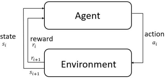
Figure1.1 shows the loop of agent-environment interaction. In a loop of agent-environment interaction, the agent observes the state of the environment then selects an action according to its policy. After the selected action has been executed, the state of the environment is changed. Meanwhile, the reward function gives a number by which to evaluate the performance of the action. Then, the agent goes to the next loop, observing the environment again and so on.
1.2. Research Gap 3
Figure 1.1: Agent environment interaction
state is the sign that the task has come to an end. For instance, in a chess game, the opponent could be considered to be like the environment. An action is represented by the making of one move during the game. If one side’s King has been checkmated, then the agent has achieved the terminal state for he has won the game and thus the task has come to an end. Obviously, however, losing pieces in the same game of chess is not good. Therefore, an agent should be given a negative reward when it loses pieces. If the agent takes the opponent’s pieces, it should be given a positive reward. A big positive reward should be given to an agent if it checkmates the opponent’s King. The environment represents the real world, like the rules and opponents in a game. The reward function, defined by humans, represents subjective wishes, the goal of a task, for example, to checkmate the opponent’s King.
1.2
Research Gap
Although the framework and perspective of reinforcement learning is very ambitious, RL algo-rithms still face many challenges:
1.2.1
Delayed feedback and credit allocation
The goal of RL is to find an optimal policy that maximises the expectation of cumulative rewards. The agent only gets the cumulative reward at the end of an episode. However,
long-4 Chapter 1. Introduction
delayed rewards make it extremely hard to trace back what sequence of actions contributed to giving of the rewards. RL needs a mechanism to allocate the total reward of a trajectory into each state-action in the trajectory. This mechanism has been called the credit allocation problem (Sutton, 1988). The details of this are discussed in Chapter two.
1.2.2
Representation of state space
Like supervised learning, RL faces the challenge of the curse of dimensionality (Bellman, 2015). In a toy task, the number of states is small and all states can be stored in one tabulation, called tabular RL. However, the number of states increases exponentially with the number of features. When it comes to a complex task, the number of features is too large to store all the states in a Q-table. Furthermore, if state features are continuous, the number of states is infinite. Function approximation techniques are used to deal above issues. It uses parameterized models of features to fit the values. Current years, Deep learning is one active research area which used an artificial neural network (ANN) to propose an end-to-end learning system which could use raw data, such as images, as input data and thereafter learn the features of the raw data via multiple level transformation. Reinforcement learning combines with deep learning is called deep reinforcement learning (DRL) in literature.
Due to the fact that the sample of RL came from trajectories, those samples were highly related. To satisfy the condition of independent and identically distributed (I.I.D) samples, memory replay has been proposed. The memory replacement technique addresses the challenge of correlation of samples by using a buffer to collect each sample online, and then resamples a batch sample from memory to fit the model. Memory replay breaks the sequential relationships of samples - Chapter Two gives more review details.
DRL has achieves some success in lots of domain. The most successful example of deep rein-forcement learning is from Google DeepMind, which invented the deep q-learning method to play the Atari Game 2600 from an image without prior knowledge. It used raw images (80x80 pixels) as input states, with multiple levels of convolutional and full connection neural networks as function approximations to learn the optimal actions performed in the game. Mnih et al.
1.2. Research Gap 5
(2013, 2015) and Hessel et al. (2017) showed that after millions of steps the agent outperformed human players in a majority of games. This was the first implemented end-to-end model-free control (reinforcement learning from raw data). After Mnih et al. (2013, 2015), Atari Game 2600 became a new benchmark for reinforcement learning research.
1.2.3
Explore and exploit the balance
An agent has no prior knowledge of a task, it only estimates and improves its model of Q-values or agent’s policy from samples. Therefore, the agent faces an explore-exploit dilemma.
Demonstrations from external experts or agent itself could be used to guide the agent with biased exploration. Chapter 3 will review previous research in this topic and chapter 4 chapter, chapter 5 and 6 shows our contributions of this area.
The key contribution of this study is biased exploration using demonstrations from inside and outside sub-optimal policies.
1.2.4
Sample inefficiency
Reinforcement learning generates samples from agent-environment interactions and then uses these samples to estimate and improve the policy. In the original reinforcement learning al-gorithm, the sample is used only once and then discarded. It follows, that information about the sample has not been completely employed. As we know, interacting with the environment involves computation time and energy costs, so improving sample efficiency is a key research topic in RL.
An off-policy RL algorithm learns the value of the optimal policy independently of the agent’s policy. Therefore, with off-policy learning, samples can be reused multiple times to increase the utilisation rate of samples.
6 Chapter 1. Introduction
1.2.5
Sparse Rewards
In most tasks, the reward of most state-action pairs is zero. This phenomenon has been called ’sparse rewards’ (Osband et al., 2014, 2016). Due to the lack of feedback from the environment, the RL agent needs to explore for a long time to find the optimal policy. Intuitively, we can add extra signals to reward or punish the agent during its learning. Changing the reward function has been called reward shaping (Ng et al., 1999). However, a change of reward function may result in a different optimal policy. For instance, a tasks only have one positive rewards, when the agent approaches the terminal state and rewards 0 for all non-terminal states. If we simply give an extra reward for a non-terminal but good state, the optimal policy will change. In such an instance, the agent will learn a policy to repeatedly enter and leave the state with extra reward rather move forward to the terminal state. This is because continually going in and leaving the extra reward state is a better choice than only getting a one-time reward.
1.3
Research Motivation
Improving the efficiency of samples is the main research focus of this thesis. One method to address this issue is guiding the RL agent to biased exploration of the state-action space with demonstration. As far as we know, all current research in this area has focused on using demonstrations from human players to guide the agent to biased exploration. In our research, we consider that demonstrations could come from the agent’s own performance in the RL loop. A filter has been applied to select qualified demonstrations to reuse. The filter will keep Currently superior demonstrations and sweep out poor demonstrations. As the agent learn from environment, the performance of demonstrations in filter have been improved continuously and finally converge into optimal demonstrations.
Conflicts between demonstrations from different resources have been ignored in some research. This thesis, therefore, focuses on how to improve the sample efficiency via demonstrations. The demonstrations come from agent-environment interactions or human experts. It has following characteristics:
1.4. Hypotheses 7
1. Sub-optimal A human expert is not an optimal agent, so the demonstration data we collected is not optimal, but is much better than random policies.
2. Conflict: For demonstrations coming from multiple sources, in a same state, it may have multiple demonstrations have different actions.
3. High-dimensional: In recent years, the deep learning technique has been introduced to re-inforcement learning. It uses raw data as a state. The demonstration data may, therefore, develop a high-dimensional raw dataset.
4. Huge size: The cost of data collection continues to reduce. For instance, numerous game corporations have collected a bulk of player behaviour data. That data could be used to help train the agent to perform a complex task.
5. Imbalanced: Demonstrations may be imbalance that major demonstration distributed on part of state space.
Considering these characteristics, we think there is a research gap that requires the building of an algorithm to deal with the challenges.
1.4
Hypotheses
In this thesis, the following hypotheses are proposed:
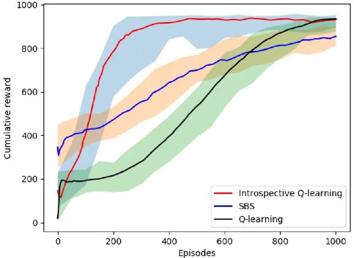
1. In Q-learning, experience samples and demonstrations can be filtered and reused to speed up the learning process via reward shaping compared the performance of state-of-art algorithm such as similarity based shaping (SBS) (Brys et al., 2015) on Super Mario Bro and cartpole.
2. An agent using a Two-level Q-learning approach will improve the performance when dealing with conflicting demonstration with sub-optimal experts, compared to state of the art Reinforcement learning from demonstrations (RLfD) method such as Confidence Human Agent Transfer(CHAT) (Wang and Taylor, 2017).
8 Chapter 1. Introduction
3. Constraining the distance between state and demonstration, called as radius in this thesis when selecting demonstrations and derive a policy from majority voting improves the performance compared to state-of-art approaches such as SBS and kNN-transfer (Wang et al., 2018).
The following assumptions are made in this thesis: The demonstration dataset is sub-optimal. The performance of the polices which produce the demonstration are better than the perfor-mance of a uniformly and randomly chosen policy.
1.5
Contribution
1.5.1
Introspective Q-learning
To deal with the sample inefficiency problem, this thesis extends the technique in Brys et al. (2015) which used Gaussian similarity between state and demonstrations to reshape the reward function. Brys et al. (2015) is based on the assume that similar states have the same optimal action and that these widely exist in many domains such as control tasks. Our approach, Introspective Q-learning succeed this assumption.
In Brys et al. (2015), the demonstrations come from human experts. However, in this research, high value samples generated during learning were considered to be demonstrations. Monte Carlo method has been used to estimate the Q-value of each demonstrations. Demonstration is recorded as a triple, noted as < st, at,Qˆt >. The triples were filtered using a priority queue.
This filter keeps high estimate values as demonstrations and keeps weeding out low value items to improve the qualification of the demonstrations. As time goes by, the triple that was kept in the filter had a high estimated value.
Introspective Q-learning is different from T D(λ) algorithm. T D(λ) algorithm propagate TD error to previous samples in a same trajectory (vertical propagation). The hyper-parameter
Intro-1.5. Contribution 9
spective Q-learning propagates values around state-actions through reward shaping and can be considered to be lateral propagation, propagating information to the surrounding state-action. Due to filter updates, the demonstration during the learning process, at the end, the agent only keeps samples from the optimal policy. Therefore, introspective RL could converge into the same optimal action as normal Q-learning.
1.5.2
RL from conflicting demonstrations
Demonstrations from multiple sources such as human experts, heuristic rules and policy trans-ferred from other domains and so on, may be in conflict (Li and Kudenko, 2018). This means that there can be multiple demonstration that have same state but possess different actions. If we ignore those conflicts, the agent cannot know which demonstrations to trust. To address conflicting demonstrations, a novel algorithm named Two-level Q-learning (TLQL) is proposed. The key idea of TLQL is that the agent learns not only the optimal policy for selecting actions, but also learns a policy of selecting which demonstrations to follow for every state.
1.5.3
RL from massive and imbalanced demonstrations
In the same domain (e.g. online games), there are a massive number of demonstrations available. This brings about two challenges. First, the distribution of demonstrations is imbalanced which means there are massive demonstrations in some particular states while there are no available demonstrations in some states. If the agent only applies its nearest demonstrations, it will tend to have the overfitting issue in the sparse demonstration regions. Second, for the states with massive demonstrations, demonstrations cover all types of actions and are in conflict. The TLQL algorithm proposed in this chapter which can narrow the action space, is not suitable for massive demonstrations.
To deal with the challenges mentioned above, a radius-restricted weighted vote algorithm (RRWV) is proposed. This approach introduces a hyper-parameter radius to select demonstra-tion candidates. The selected demonstrademonstra-tion candidates then vote for demonstrademonstra-tions’ acdemonstra-tions.
10 Chapter 1. Introduction
In the algorithm, votes on each action are counted and a policy via softmax function on the votes is produced accordingly. Compared with previous studies on RL with demonstrations, our approach provides new techniques to address complicated demonstration settings.
1.6
Structure of the Thesis
As Figure 1.6 illustrations, this thesis is separated into six chapters.
Chapter Two reviews the definitions of the Markov decision process, terminology, and math-ematical notations. This chapter also reviews the classic algorithm to evaluate and improve the policy via state-action value. Policy gradient algorithms and derivative algorithms are also included. Current reinforcement learning is well developed, combined with deep learning. In Chapter Two, we review deep Q-learning and its derivative algorithms: Double-DQN, Dual-DQN, prioritised replay, noise DQN. The policy gradient method and value function base are combined in an actor-critic framework. State-of-the-art techniques, such as TROP and PPO, are also included in this chapter.
Chapter Three is a review of related research in which external information to speed up the RL process is used. External information could come from human expert demonstrations, heuristic rules, online agents advising, and transferring policy from other tasks. In this chapter, we review the characteristics of the external information sources. How to combine RL with that information is a well-studied research topic, and there are some techniques to inject external information into RL loops, such as reward shaping, probability reuse, pseudo-action and so on. These are reviewed and commented upon.
Three classes of methodology pertaining to injecting human expert demonstrations into the agent’s learning process are reviewed first. We also review behaviour clones and human-involved agent-environment interactions. Finally, discussions on the differences between that research and the work in this thesis is presented.
1.6. Structure of the Thesis 11
Figure 1.2: Thesis structure
the introspective RL algorithm works. It applies a priority queue to filter high-value samples during the learning process and uses the reward shaping technique to supply extra reward signals to the agent.
Chapter Five: Q-learning with multiple conflicting demonstrations, describes the technique details of Q-learning with multiple conflicting demonstrations. This novel method can make an agent not only learn the policy of selecting actions, but also select experts to trust in.
In Chapter Six, we study and analyse reinforcement learning from a mass demonstration setting. It proposes to derive a policy from demonstrations with a radius. This technique helps avoid over-fitting in sparse demonstration regions. It also addresses demonstration conflicting issues via softmax voting weighted by Gaussian distance.
In the final chapter, conclusions are drawn based on our work. In addition, this chapter also presents further research directions drawing on the work presented in the thesis.
12 Chapter 1. Introduction
1.7
Chapter Summary
In this chapter, an overview of reinforcement learning has been given. In addition, this chapter has identified that improving sample efficiency is one of the challenges and difficult issues faced by reinforcement learning. Existent research gaps and our hypotheses were also presented in this chapter. Finally, the contributions that this thesis makes to the furtherance of existing academic knowledge were noted as well as an overview of the thesis’ structure.
Chapter 2
Reinforcement Learning Background
In this chapter, we provide the background to reinforcement learning and define the terminology used in later chapters. We also review state-of-the-art algorithms in RL that are compatible with deep neural networks.
2.1
Overview
Reinforcement learning (RL) is a paradigm of a behavioural learning model (Sutton et al., 1998). The RL agent receives feedback from the environment, guiding the agent to the optimal policy. Unlike other types of supervised learning, RL is not trained on labelled training data, but learns a policy via receiving a reward signal on each step. The solution to the task, called ‘the policy’, is defined as a mapping from the state space to the action space, denoted as π(s) (Szepesvári, 2010; Wiskott, 2016). Unlike the one-shot decision of supervised learning, the goal of RL is to search for an optimal policy to gain the maximum accumulated reward from the whole trajectory. RL is a memoryless process that can be modelled, as described in the next section, as a Markov Decision Process (MDP).
Early research included applying RL to classical control problems such as mountain-car (Boyan and Moore, 1995), cartpole (Geva and Sitte, 1993) and pendulum (Anderson, 1989). Tesauro
14 Chapter 2. Reinforcement Learning Background
(1995) trained an RL agent, TD-Gammon, to play Backgammon. After a simulation with self-play, it was able to beat a human backgammon champion. The past thirty years have seen tremendous achievements in the field of RL. In 2015, Google DeepMind proposed a Go player agent, AlphaGo (Silver et al., 2016), and beat the top ranked human player. This attracted wide public attention to the progress that had been made in the field of RL. Following this, AlphaGo combined various techniques such as deep learning, Monte Carlo Tree search and memory replay as a general solution to board games and cards. This solution was called Alpha zero (Silver et al., 2017b), and it won shoji (Japanese chess) (Silver et al., 2017a) and other games. RL also achieved successes in other domains such as Dota (OpenAI, 2018), finance (Nevmyvaka et al., 2006; Van Roy, 2001), recommendations (Golovin and Rahm, 2004), and robotics (Kober and Peters, 2012).
2.2
The Markov Process
Markov processes are the foundation of RL. This chapter introduces Markov Chains, Markov Reward Processes and, Markov Decision Processes.
2.2.1
Markov Chains
A Markov Process or Markov chain is a memoryless process which is represented as two-tuples ⟨S, T⟩. S is a set of states, represented as a vector; T is a transition probability matrix of states. If the probability of the current state depends only on the probability of the previous state, it is regarded as having a Markov property (Kaelbling et al., 1996). Markov processes can be described by equation 2.1:
Ps,s′ =P[St+1 =s′|St =s] (2.1)
Markov properties were introduced to model the environment-agent interactions because RL is a memoryless process. For a finite state set S, the transition function T can be expressed as a
2.2. The Markov Process 15
matrix shown in equation 2.2 V(s1|s1) T(s2|s1) ... V(sn|s1) V(s1|s2) T(s2|s2) ... V(sn|s2) ... V(s1|sn) T(s1|sn) ... V(s3|sn) (2.2)
2.2.2
The Markov Reward Process
A Markov reward process (MRP) consists of a reward function and a Markov chain. The reward function is a utility function which maps from a< state, action >pair to a real number, noted as
R(s, a)7→R. A positive reward means an award is given whereas a negative reward represents a punishment. The cumulative reward is a discounted sum of rewards from time step t to the horizon.
Gt =rt+γrt+1+γ2rt+2+... (2.3)
Equation 2.4 defines the value of state as the expected return from the start in state s noted as:
V(s) =E[rt+γrt+1+γ2rt+2+...] (2.4)
γ is a hyper-parameter, a real number between 0 and 1, to balance the short-term reward and the long-term reward. If the discount is 0, the agent only learns the reward of one step; this is equivalent supervised learning. If the discount is 1, all rewards in the present and in the long term are considered to be equally important.
2.2.3
The Markov Decision Process
A Markov Decision Process (MDP) is defined as a five-tuple (S, A, R, T, γ). Specifically, A is the action space in which an agent interacts with the environment. The policyπ of a RL agent
16 Chapter 2. Reinforcement Learning Background
is a mapping from a state-action to a probability, denoted as π : (S, A) 7→ [0..1]. Applying the policy π in the MDP results in a Markov Reward Process (MRP) (S, A, Tπ, Rπ, γ) where
Rπ(s′|s) = ∑
a∈Aπ(a|s)T(s′|s, a), T
π(s′|s) = ∑
a∈Aπ(a|s)T(s′|s, a). Equation 2.5 shows the
Bellman equation, which is the foundation of dynamic programming and temporal difference algorithms.
Vπ(s) =Rπ(s) +Tπ(s′|s)Vπ(s′) (2.5)
Equation 2.5 indicates that a MDP can be decomposed into sub-problems. These sub-problems can be reused in the algorithm.
2.3
Model-based policy estimation
The term ‘model-based’ used here refers to a setting in which the transition probability function is known. Because of this, both the analytical solution and the iterative algorithm can be applied to solve the task.
According to the definition of a state value, it can be decomposed into two parts: the immediate reward and the discounted sum of future reward: V(s) =R(s) +γ∑T(s′|s). The finite states of a MRP could be expressed as the matrix below:
Tπ(s 1) Tπ(s2) ... Tπ(s N) = Rπ(s 1) Rπ(s2) ... Rπ(s N) +γ Tπ(s 1|s1) ... Tπ(sn|s1) Tπ(s1|s2) ... Tπ(sn|s2) ... Tπ(s 1|sn) ... Tπ(s3|sn) Vπ(s 1) Vπ(s2) ... Vπ(s N) (2.6)
2.4. Model-free policy estimation 17
Vπ−γTπVπ =Rπ
(I−γTπ)V =R Vπ = (I−γTπ)−1Rπ
(2.7)
The computational complexity of this solution is O(N3), as a matrix inverse operation was
involved.
Dynamic programming is another solution through iteration, as shown by Algorithm 1. The computational complexity of the dynamic programming is O(N2) for each iteration.
Algorithm 1 Dynamic programming of MRP
procedure Dynamic programming of MRP under policy π
for k=1 until convergence do:
for all s in S do: Vπ k(s) = Rπ(s) +γ ∑ s′∈ST π(s′|s)Vπ k−1(s′) end for end for end procedure
2.4
Model-free policy estimation
In most circumstances, the transition probability function is unknown or is too complex to be represented. Model-free estimation does not require a known transition function (Sutton et al., 1998). Rather, it estimates the expectation of state values by sampling data through agent-environment interactions.
2.4.1
The Monte Carlo estimation
Monte Carlo techniques (MC) estimate the expectations of state values using rewards from trajectories as Algorithm 2 shows.
18 Chapter 2. Reinforcement Learning Background
Algorithm 2 Monte Carlo model-free estimation
procedure General policy iteration
for each state s visited in episode i do: total first visits N(s) = N(s) + 1
Increment total return S(s) =S(s) +Gi,t
Update estimate Vπ =S(s)/N(s)
end for end procedure
The process of mean estimation can be incremental.
Vπ(s) =VπN(s)−1 N(s) + Git N(s) =V π+ 1 N(s)(Git−V π(s)) (2.8)
The α is defined as a learning step in the MC estimation:
• α= N1(s) is identical to every MC visit.
• α > N1(s) opens a memory window to forget older samples. This is useful in non-stationary domains. Vπ(s) =VπN(s)−1 N(s) + Git N(s) =V π+α(G it−Vπ(s)) (2.9)
Due to the fact that MC estimates the cumulative reward from the whole episodes, it does not require either Markov properties or the known transition function. Although MC is an unbiased estimation of the policy value, the variance of trajectory samples is very large, especially in tasks with a long trajectory. MC needs numerous samples from a complete trajectory to confidently predict an estimated value.
2.4.2
Temporal difference estimation
Temporal difference learning (TD) adheres to the properties of MDPs, and reuse the estimated value of the next state to estimate the value of the current state. It is called the bootstrap
2.5. Policy improvement 19
technique. TD estimates the cumulative reward of the trajectory Gt byγVπ(St)plus one-step
reward rt. Therefore, unlike the MC, the TD is a biased estimation of the policy value.
Vπ(s) =Vπ +α([rt+γVπ(st+1)]−Vπ(s)) (2.10)
The Vπ(s)is called the TD prediction, andR
t(s) +γVπ(st+1)refers to the TD target. The TD
error will be continuously reduced until the agent approaches an acceptable performance level.
Compared with MC, TD algorithms have a number of benefits. First, the TD algorithm updates the value step-by-step, while the MC updates the value trajectory by trajectory. This means the TD does not require the task to have a finite horizon. With the discount of less than 1 , an infinite-horizon task also converges to its state value. Second, with the bootstrap technique in the TD, variance is reduced. Theoretically, the TD algorithm will converge to a true state value when every state is visited unlimited times, according to the law of large number.
2.5
Policy improvement
2.5.1
Generalised policy improvement
The goal of RL is to find an optimal policy so as to obtain the maximum cumulative reward.
π∗(s) = arg max
π V
π(s) (2.11)
In reality, however, the policy space is extraordinarily large. For instance, even when the state set S and action set A are finite and discrete sets, the size of policy space will be |A||S|.
To use the principle of Bellman equation, state values V are decomposed into Q-values of
20 Chapter 2. Reinforcement Learning Background
reward plus theV value of the next state following the policy.
Qπ(s, a) =R(s, a) +γ∑
s′∈S
T(s′|s)Vπ(s′) (2.12)
The policy πi on state s could be monotonously improved toπi+1 by a maximisation operation
as Equation 2.13 shows. max a Q πi+1(s, a) = max a R(s, a) +γ ∑ s′∈S T(s′|s, a)Vπi(s′) ≥Rπ(s) +γ∑ s′∈S Tπ(s′|s)Vπi(s′) (2.13)
Model-free policy search is a contextual multi-armed bandit problem that needs an exploration-exploitation balance. In this thesis, we use the ϵ −greedy strategy to improve the policy. Greedy here means that the agent applies the current policy by selecting the action with the maximum Q-value. To balance exploration and exploitation, the agent randomly chooses an action with a uniform distribution under a small probability ϵ. Algorithm 3, which combines policy evaluation and policy improvement, is called the generalised policy iteration (GPI); it facilitates the convergence to the optimal policy.
Algorithm 3 Generalised policy iteration
procedure Generalised policy iteration
while i==0 or |πi−πi−1|>0 do:
policy estimation: Vπi
policy improvement: πi+1 =ϵ−greedy(Vπi)
end while end procedure
Policy estimation and policy improvement can operate in one iteration, called the value itera-tion, as Algorithm 4 shows.
2.5. Policy improvement 21
Algorithm 4 Value interaction
procedure Dynamic programming of MRP under policy π
while ∆< θ do: ∆ = 0 for all s in S do: v ←V(s) V(s)←maxa ∑ s′T(s′|s, a)[r+γV(s′)] ∆←max(∆,|v−V(s)|) end for end while end procedure
2.5.2
TD-learning
TD-learning follows the same structure as the value interaction algorithm (Algorithm 4). In-stead of interacting with a known transition function, the TD-learning agent estimates and updates the value function with samples. For each sample, the Q-value is then updated by the temporal difference error (TD-error) between the target Q-valueR+γQ(s′, a′)and the current Q-value Q(s, a).
SARSA
State-Action-Reward-State-Action (SARSA) (Rummery and Niranjan, 1994) is a model-free and on-policy algorithm that can update the policy based on the action from its current policy. With an exploration-exploitation balance like ϵ-greedy, SARAS selects action a from s using the policy derived from the Q-value function. The updated SARSA rule is:
Q(s, a)←Q(s, a) +α[R+γQ(s′, a′)−Q(s, a)]
Q-learning
Q-learning is an off-policy algorithm because the policy generating samples and the policy being updated are different. The policy generating samples is derived from the Q-value function via
22 Chapter 2. Reinforcement Learning Background
Q-value with TD-error between the current Q-value: Q(s, a) and the target Q-value: R + maxaγQ(s′, a). The updated Q-learning rule is:
Q(s, a)←Q(s, a) +α[R+ max
a γQ(s
′, a)−Q(s, a)]
Eligibility Traces
TD-learning can reduce variance using bootstrapping samples. However, it is a biased estima-tion of true value. Monte Carlo, on the other hand, is an unbiased estimaestima-tion but has variance. An eligibility trace (Sutton et al., 1998; Kaelbling et al., 1996) can mix both TD-learning and MC. The integration of TD-learning and MC can be recognised as a special case of an eligibility trace.
An eligibility trace can record the previously experienced occurrences of state-action pairs. Samples from environment interaction is recorded in the trace with an eligibility of one. In an eligibility trace, a hyper-parameter λ, where 0 < λ < 1 is introduced as the decay rate. The eligibility of samples is decayed by multiplication withλ. The eligibility trace algorithm remove samples that less than a threshold. Only state-action pairs in the trace are updated when a reward is received. If λ= 0, the TD(0) will be equal to the TD algorithm, because it only has a one-step update. However, when λ= 1, it will update the Q-value using a discounted sum of rewards in the whole trajectory; this is equivalent to the Monte Carlo approach. An eligibility trace for the state s and action ais updated as follows:
e(s, a) =← 1 s =at, a=at γλ(s, a) otherwise
An eligibility trace can be presented as a vector e. The parameters of the Q-value approxima-tion, θ, is updated based on Equation 2.14, where δ denotes the TD-error between the target value and the current value.
2.6. Function approximation 23
θ ←θ+αeδ (2.14)
2.6
Function approximation
When the domain is small, a look-up table can store all state-action pairs (Busoniu et al., 2010). However, the size of the look-up table grows exponentially with the number of state features. Bellman (1961) called this phenomenon ’the curse of dimensionality’. Due to the limitation of memory and computational time, a tabular representation cannot hold a complex task and a function approximation must be involved. In addition, for continuous state and action spaces, a look-up table is not suitable because the number of state-action pairs is infinite.
The first step of a function approximation is to represent the state-action pairs as features. This is denoted as in the equation 2.15.
X(s, a) = X1(s, a) X2(s, a) ... Xn(s, a) (2.15)
The goal of a function approximation is to minimise the loss error between the true state-action value function Qπ(s, a) and the approximate state-action value functionQˆπ(s, a,w). w
is parameters to learn. The loss function is defined through the approach noted in equation 2.16:
J(w) =Eπ[(Qπ(s, a)−Qˆπ(s, a,w))2] (2.16)
In TD-learning, TD-error is used as the loss function, as shown in equation 2.17. Weight w is updated according to its gradient∇JT D(w) as equation 2.19 and 2.18 shows.
JT D(w) =
1
2(r+γmaxa′ ˆ
24 Chapter 2. Reinforcement Learning Background
∇JT D(w) = (r+γmaxa′Qˆ(s′, a′,w)−Qˆ(s, a,w))∇wQˆ(s, a,w) (2.18)
w=w+∇JT D(w) (2.19)
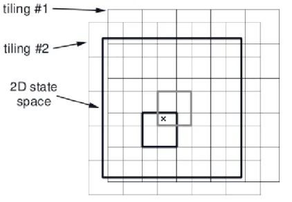
In this thesis, tile coding and deep neural network were employed as function approximators. Tile coding is a piece-wise constant approximation that is particularly well suited for continuous state space (Sutton et al., 1998). In tile coding, the feature space is grouped into partitions. As Figure 2.1 shows, each partition is defined as a tiling and each item in the partition is a tile. Each tile is represented with binary features. If the given state falls into the region represented by a tile, the binary record is 1. If not, the record is 0. The state value represented via tile coding is the sum of weights:
V(s) =
n
∑
i=1
bi(s)wi (2.20)
where n is the number of tiles; bi(s)is record of the ith tile; and, wi is the weight of each tile.
The gradient of the value function is:
∇V(s) = max
a (R(s, a) +γV(s
′))−V(s)
The updated rule is:
wi ←wi+
α
mbi(s)∇V(s)
Smaller tiles produce fewer approximation errors but their generalisation abilities are reduced. Adding more layers of tiling can improve the precision of learning. The number of tiles is defined as a hyper-parameter that can be used to balance learning speed and precision (Whiteson et al., 2007).
2.6. Function approximation 25
Figure 2.1: Tile coding (Sutton et al., 1998)
2.6.1
Deep Reinforcement learning
Deep learning is a type of machine learning method based on learning data representations, as opposed to task-specific algorithms with feature engineering. In a general way, it is based on the layers used in artificial neural networks (ANNs) (Bengio et al., 2009). Deep learning and RL are integrated in Deep Reinforcement learning (DRL), which has been developed rapidly since 2015 when Mnih et al. (2015), proposed an end-to-end player agent to Atari. In this chapter, Deep Reinforcement Learning (DRL) and its derivation algorithms are introduced.
Deep Q-learning
ANNs are models vaguely inspired by the biological neural networks in human brains (Schmid-huber, 2015). Classic techniques, such as the Multi-layer Perceptron (MLP) and the Convo-lutional Neural Networks (CNN), were well developed in the 1980s and the 1990s. Benefiting from data blooming and the increase in computational power today, ANN techniques have been revived in the past decade. AlexNet (Krizhevsky et al., 2012) shows that the deep learning CNN to have high power in the ImageNet competition. CNNs use filters to detect margin infor-mation from images and automatically extract features using multiple iterations of convolution operations. This process is called end-to-end learning or representation learning.
26 Chapter 2. Reinforcement Learning Background
The integration of RL with an ANN was examined in earlier research. Riedmiller (2005) first applied an ANN to fit Q-values. Lange et al. (2012) proposed the deep fitted Q-Learning(DFQ) algorithm to build a vehicle control system. Mnih et al. (2013, 2015) combined Q-learning and the CNN technique to use raw pixels as input and produce the Q-values of actions. This was the first end-to-end control system, which outperformed human expert players in most Atari 2600 games. AlphaGo is a Go play agent which defeated the human champion Lee Se-dol and demonstrates the power of deep reinforcement learning.
In Mnih et al. (2013), the inputs to the Deep Q-Network (DQN) include the last 4 frames of images. The transition of images was via 3 layers of a CNN, and then 2 fully-connected layers which produced Q-values for each action. Another important contribution of DQN is memory replay. Function approximation must assume that training data satisfies independent and identically distributed (I.I.D) sampling. However, in Q-learning, data comes from episodes of interactions. Step samples from the same episode are strongly related. To break the correlations of samples, DQN introduces a replay buffer called memory to collect samples deriving from interactions and re-sample batches of datasets from memory to train the neural network. The vanilla DQN is shown in Algorithm 5
Algorithm 5 Vanilla DQN
procedure DQN
Initialise Q-netθ,target-Q-net θ, Memory D.
for episode=1...M do for t=1...Tdo
exploit-explore with Q-netθ′
store transition < st, at, rt, st+1 > into D
sampling minibatch of transitions from D setyi =
{
rj if terminate at j+1
rj+γmaxa′Qˆ(ϕj+1, a′;θ) otherwise
perform a gradient descent ofθ on(yj−Q(ϕj, aj;θ))2
end for end for end procedure
2.6. Function approximation 27
2.6.2
Improvement of DQN
After the great success of Mnih et al. (2013), different types of DQN modified algorithms have been proposed in the last three years to improve its performance from different perspectives. The following algorithms are the most influential.
Target net Freeze
In Mnih et al. (2013), the agent updates the neural network after each interaction. To avoid oscillations of the neural network in small sets of samples, Mnih et al. (2015) introduced a network freezing technique to separate the Q-network into two identical nets called current net and target net. The target network provides actions during the learning process and the parameters of the current network are optimised at every step. After N updates (N is a hyper-parameter), the parameters of the current Q-network are copied to the target Q-network. Therefore, compared with the vanilla DQN, the policy updating frequency is decreased and the algorithm is more stable (Mnih et al., 2015).
Double DQN
Using anϵ−greedy policy to estimate the Q-value yields a maximisation bias (Hasselt, 2010). To avoid the bias, Van Hasselt et al. (2016) applied two independent networks to the unbiased estimation of Q-values. One Q-network, noted asQ1was applied to select an action and another
Q-network, noted as noted as Q2 was employed to estimate the target Q-value alternatively as
Equation 2.21 shows. Q(s, a) =Q2(s,arg max a Q1(si, a)) Q(s, a) =Q1(s,arg max a Q2(si, a)) (2.21)
28 Chapter 2. Reinforcement Learning Background
Figure 2.2: A popular single stream Q-network (top) and the dueling Q-network (bottom) (Wang et al., 2015)
Dueling DQN
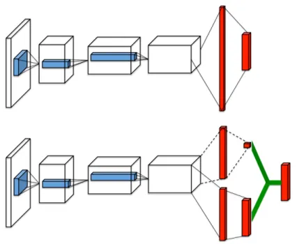
In some domains, such as Atari game Enduro, actions do not affect the environment in a relevant way (Wang et al., 2015). Therefore, calculating values of state-action pairs is unnecessary. Dueling DQN (Wang et al., 2015) estimates the state-dependent action advantage function rather the Q-value function of state-action pairs. The advantage function of (s, a) pairs is defined as:
Aπ(s, a) = Qπ(s, a)−Vπ(s)
As figure 2.2 shows, the value of stateVπ(s)and the advantage of the state-actionAπ(s, a)are
decoupled into two output tensors in the neural network. Through the decoupling, the DQN agent can learn which states are valuable without learning the effect of each action on each state.
Memory prioritised replay
The idea of memory prioritised replay is that some samples in memory should be more impor-tant than others. However, these more imporimpor-tant samples might be selected less frequently. In
2.6. Function approximation 29
vanilla DQN, the agent re-samples steps from its memory using a uniform distribution. Schaul et al. (2015) considered that the agent should extract samples from memory using different weights. The TD-error indicates how surprising the sample is. Therefore, high TD-error tran-sitions should be sampled with high probabilities. Schaul et al. (2015) re-organised samples in memory using a priority queue. Each sample in the priority queue was selected based on its priority.
Distributional DQN
The key idea of Distributional DQN (Bellemare et al., 2017) is to model the distribution of the cumulative reward rather than to model the expected value. If the environment is stochastic and the Q-value follows a multimodal distribution (e.g. bi-modal distribution), the action from arg maxa(s, a) may lead to a sub-optimal outcome. The authors proposed the distributional
Bellman equation, as shown in Equation 2.22. This uses Z(s, a) to replace Q(s, a) in the Bellman equation. Z(s, a)is the distribution of the cumulative reward. The Wasserstein Metric is applied to measure the distance between Z(s, a) and R(s, a) +γZ(s′, a′). Bellemare et al. (2017) given the mathematical proof of the convergence of the distributional Bellman equation.
Z(s, a)=D R(s, a) +γZ(s′, a′) (2.22)
There are two main benefits of the Distributional DQN. Firstly, the agent can take the distribu-tion of Q-value into account in selecting an acdistribu-tion rather than considering only the maximum Q-value. Secondly, even if the expected cumulative rewards are the same, their variances might be very different. In the literature on finance, the variance is regarded as the risk; people are generally risk-averse which means that actions with lower variances should be selected, if their expected values are the same.
Noisy DQN
30 Chapter 2. Reinforcement Learning Background
noise to the neural network. This is a new approach to balance exploration and exploitation. Compared with ϵ−greedy, the noisy network could yield substantially higher scores for a wide range of Atari games.
Rainbow
Hessel et al. (2017) examined 7 scaling DRL algorithms in Atari Games. The combination of all 7 improved techniques outperformed each algorithm. Hessel et al. (2017) provided an overview of the current development of DQN. DQN is the general framework for optimal control with raw data. This algorithm can improve a good performance in most of the 57 Atari games, but not in every game. The games that are unable to benefit from DQN in Atari, such Montezuma’s Revenge, indicate that learning without knowledge has limitations under some circumstances. DQN and its improved algorithms have a low sampling efficiency. For example, the DQN agent needs to learn over 4 million frame images to approach the optimal policy in Atari games. In a real application, samples are limited because of the scarce resources of agent-environment interactions. Therefore, reducing the number of interactions with the environment is one of the pressing topics in the field of DRL.
2.7
Policy gradient
Another approach in RL is to directly search for the policy with a maximised cumulative reward. Compared with value-based approaches, policy gradient algorithms do not keep the value function. The parameterised policy is able to deal with continuous state space and action space. Policy gradient algorithms regard RL as an optimisation problem.
2.7.1
REINFORCE
Note the policy as πθ(s). τ denotes the episode, a state-action sequence < s0, a0 > ... <
sH, aH >. The definition of cumulative reward is R(τ) =
∑H
2.7. Policy gradient 31
methods, the goal of RL is to find a parameter θ that can maximise the expectation of the cumulative reward of episodes, which is defined by equation 2.23:
θ = arg max
θ
∑
τ
P(τ;θ)R(τ) (2.23)
The parameters of the policy, θ, can be optimised by gradient ascent methods. The gradient w.r.t θ is defined as Equation 2.24: ∇θπθ =∇θ ∑ τ P(τ;θ)R(τ) =∑ τ ∇θP(τ;θ)R(τ) =∑ τ P(τ;θ) P(τ;θ)∇θP(τ;θ)R(τ) =∑ τ ∇θP(τ;θ) ∇θP(τ;θ) P(τ;θ) R(τ) =∑ τ P(τ;θ)∇θlogP(τ;θ)R(τ) ≈ 1 m m ∑ i=1 ∑ τ P(τ;θ)∇θlogP(τ;θ)R(τ) (2.24)
REINFORCE (Williams, 1992) is an earlier algorithm for gradient descent methods. It can generate an episode with policyπ(a|s, θ). For each episode, it uses the cumulative rewardGto derive the gradient of the current policy πθ as per Equation 2.25.
θ ←θ+αγtGt∇θlogπθ(st, at) (2.25)
2.7.2
Reducing the variance of the gradient
The weakness of using REINFORCE is the high variance of the gradient which results in unstable training. An effective method to reduce variance is to introduce a constant baseline.
32 Chapter 2. Reinforcement Learning Background
When the cumulative reward subtracts the constant, the gradient stays the same whilst the variance of the gradient can be reduced.
Proof: ∇θE[R(τ)−b] =∇θE[R(τ)]− ∇θE[R(b)] (2.26) ∇θE[R(b)] = ∇θ ∑ τ P(τ;θ)·b =b· ∇θ ∑ τ P(τ;θ) = b· ∇θ1 = b·0 = 0 (2.27)
Another method to reduce the variance of the gradient is rooted in the idea of ‘reward to go’ (Wu et al., 2018). This comes from the fact that ∇θlogπθ(a
(i)
t |s
(i)
t ) should only depend on the
step after < st, at>. The gradient∇θJ(θ) has been modified as Equation 2.28 shows.
∇θJ(θ) = 1 N N ∑ i=1 T ∑ t=1 ∇θlogπθ(a (i) t |s (i) t )Qπ(s (i) t , a (i) t ) (2.28)
2.7.3
Actor-Critic
In the REINFORCE algorithm, a whole trajectory needs to be collected to get the cumulative reward and to compute the gradient of the policy. Therefore, TD-learning can be introduced into REINFORCE to improve learning efficiency. The Actor-Critic algorithm is a strategy combining policy gradient and TD-learning.
The actor is a stochastic policy, πθ, which delivers actions to be executed. The critic,
param-eterised by w, is the value function used to estimate the value of the current policy. Figure 2.3 shows the Actor-Critic algorithm. For each < s, a >step sample from interaction with the environment, the algorithm fits the value function as Equation 2.29 shows.
minϕ(rt+1+γVϕ(st+1)−Vϕ(st))2 (2.29)