MODELING AND SIMULATION OF GRID CONNECTED PHOTOVOLTAIC DISTRIBUTED GENERATION SYSTEM

A NOVEL SQUARE ROOT CUBATURE KALMAN FILTER

USING MODEL-ENHANCED GAUSSIAN PROCESS

STATE-SPACE MODELS

ZHIKUN HE, GUANGBIN LIU, XIJING ZHAO, ZHICHENG YAO, BO ZHANG

Xi’an Research Institute of High-Tech, Xi’an, Shaanxi 710025, China

ABSTRACT

A novel nonlinear filter called model-enhanced Gaussian process square root cubature Kalman filter (MEGP-SRCKF) is proposed to estimate the state of nonlinear dynamic systems where their state-space models are unknown or insufficiently accurate. The algorithm integrates Gaussian process regression (GPR) into square root cubature Kalman filter (SRCKF). Given the training data, GPR model is used to learn and represent the residual of system after factoring the contributions of the parametric model. The combination of GPR and parametric models enhances the performance of either model alone. It improves the accuracy of the transition and measurement models. The resulting MEGP-SRCKF algorithm has several advantages over standard extended Kalman filter (EKF), nonaugmented unscented Kalman filter (UKF), augmented UKF, and SRCKF. Two cases are used to test these filters and the superiority of the proposed filter is demonstrated, where the MEGP-SRCKF can obtain the better results whether an accurate parametric state-space model is obtained.

Keywords: Bayesian Filter, Cubature Rule, Gaussian Process Regression, Model-Enhanced, Parametric Model, State-Space model, Nonlinear Dynamic System

1 INTRODUCTION

Filtering in dynamical systems is frequently used in many areas from inertial guidance of aircrafts and spacecrafts to weather and climate prediction. One of the basic problems of filtering is to process noisy measurements to obtain estimates of all of the state variables. In the case where the transition and measurement models of dynamic systems depend on the past information and when we have the assumptions that both the models in the state-space are linear and that the noise terms are normally distributed, the standard linear recursive Kalman filter algorithm can be derived [1]. The Kalman filter is a well-known recursive state estimator for linear systems. However, in many cases interesting dynamic systems are not linear by nature, and the traditional Kalman filter cannot be applied in estimating the state of such these systems. In this kind of systems, both the models can be nonlinear or only one of them.

Many nonlinear filtering methods, such as the extended Kalman filter (EKF) [2,3], the unscented Kalman filter (UKF) [4], the assumed density filter (ADF) [5], and the quadrature Kalman filter (QKF)

[6,7]

, have been proposed for filtering in dynamical systems. Based on the first order Taylor series expansion of the transition and measurement models

numerical stability, the square-root format of CKF (SRCKF) is also developed. However, like the traditional filters, the performance of CKF relies on an accurate parametric transition and measurement models, which include the properly selected process and measurement noise statistics. For many applications, the accurate parametric models are difficult to obtain. Even though such parametric models are very efficient, they often ignore hard to model aspects of dynamic systems so that their predictive capabilities may be limited.

To overcome the limitations of parametric models, we introduce non-parametric, Gaussian process regression (GPR) models to enhance the parametric transition and measurement models for dynamical systems. Meanwhile, GPR models can provide uncertainty estimates for their predictions so that they are seamlessly incorporated into Bayesian filters [10]. In this paper, we integrate GPR models into the SRCKF to enhance the parametric models. The combination of GPR and parametric models, which alleviates some of the problems with either model alone, can obtain higher prediction accuracy. The resulting filtering algorithm is thus referred to as model-enhanced Gaussian process square-root cubature Kalman filter (MEGP-SRCKF).

The rest of this paper is organized as follows. Section 2.1 gives the general filtering framework of the Bayesian filter in the Gaussian domain and Section 2.2 derives the new cubature rule for Gaussian-weighted integrals in detail. GPR method is introduced briefly in Section 3. MEGP-SRCKF algorithm is derived and its implementation is described in Section 4. Section 5 demonstrates the advantages of MEGP-SRCKF over the other traditional filters via an example. Finally, some concluding remarks are given in Section 6.

2 CUBATURE KALMAN FILTER

2.1 Bayesian filter theory in the Gaussian Domain

Consider the general state-space model with additive noise:

Transition model: xk =f(xk−1)+wk−1, (1) Measurement model: zk=h(xk)+vk, (2)

where nx

k∈R

x and nz

k∈R

z are the state and measurement of the system at discrete time k respectively; f(⋅) and h(⋅) are some known functions; w_k−1~N(0,Q_k−1) and v_k ~N(0,R_k)

are the independent process and measurement Gaussian noise with zero means and covariances

1

−

k

Q and Rk respectively.

The Gaussian distribution has many distinctive mathematical properties and it approximates many physical random phenomena, so it is the most convenient and widely used density function assumption to approximate the Bayesian filter. We call the approximate Bayesian filter as Gaussian filter. Consider the discrete-time state-space model given by Eq. (1) and (2). For this model, due to the fact that Gaussian distribution is completely specified by its mean and covariance, the general filtering framework of the Gaussian filter is given as follows [6,11]:

), ˆ ( ˆ

ˆ_k|k =x_k|k−1+W_k z_k−z_k|k−1

x , 1 | , 1 | | T k k k k k k k

k P W P W

P = − − zz −

, 1 1 | , 1 | , − − −

= _{kk kk}

k P P

W xz zz

where , ) , ˆ ; ( ) (

ˆ _|−1=

∫

₋₁ × _{−1 −1|−1 −1|−1 −1} x

n k k k k k k k

k

k _R f x x x P dx

x N (3)

, ˆ ˆ ) , ˆ ; ( ) ( ) ( 1 1 | 1 | 1 1 | 1 1 | 1 1 1 1 1 | − − − − − − − − − − − − + − × =

_∫

k T k k k k k k k k k k k T k k k d P P x n Q x x x x x x f x f N

R ₍₄₎

, ) , ˆ ; ( ) (

ˆ _{| −1}=

∫

× _{| −1 |−1}

x

n k k kk kk k

k

k _R h x x x P dx

z N (5)

, ˆ ˆ ) , ˆ ; ( ) ( ) ( 1 | 1 | 1 | 1 | 1 | , k T k k k k k k k k k k k T k k k d P P x n R + − × = − − − − −

∫

z z x x x x h x h zz N R ₍₆₎ . ˆ ˆ ) , ˆ ; ( ) ( 1 | 1 | 1 | 1 | 1 | , T k k k k k k k k k k k T k k

k nx P d

P − − − − − − × =

_∫

z x x x x x h x

xz _R N

(7)

From Eq. (3) to Eq. (7), it shows that the key of the Gaussian filter is how to compute multi-dimensional Gaussian weighted integrals whose integrands are all of the form “nonlinear × Gaussian density”.

2.2 Cubature Rule For Gaussian-Weighted Integrals

Consider a multi-dimensional Gaussian weighted integral of the form

∫

−

= _n d

I T

R f x x x x

f) ( )exp( )

( (8)

where f(⋅) is some arbitrary function. To compute Eq. (8), it is firstly converted into a spherical-radial integration form by the change of variables as follows: Let x=ry with yTy=1, so that xTx=r2 for r∈[0,∞). Then Eq. (8) can be rewritten as the radial integral

∫

∫ ∫

∞ ₋ ∞ ₋ − = − = 0 2 1 0 2 1 ) exp( ) ( ) ( ) exp( ) ( ) ( dr r r r S dr d r r r I n U n n y y f f σ (9)

1 ) ( ) ( ) ( ) ( )

(r =

∫

f ry wy d y wy ≡ S

n

U σ (10)

where Un=

{

y∈Rn|yTy=1

}

denotes the surface of the unit sphere and σ(⋅) denotes the area element on Un.

The spherical integral Eq. (9) and the radial integral Eq. (10) are numerically computed by the third-degree spherical cubature rule and the Gaussian quadrature rule, respectively. Hence, we have

[ ]

∑

= ⎟

⎟ ⎠ ⎞ ⎜ ⎜ ⎝ ⎛

≈ n

i

i n

n n

I

2

1 1 2 2

)

(f π f

where

[ ]

u represents a complete fully symmetric set of points that can be obtained by permutation and changing the sign of the generator u in all possible ways,

[ ]

ui denote the i-th point from the set

[ ]

u . For example, when n=3 and u=（1,0,0）T =（1） (zero coordinates are suppressed for brevity),

[ ] [ ]

u = 1 represents the following set of points:

[ ]

.

1 0 0 , 1 0 0 , 0

1 0 , 0 1 0 , 0 0 1 , 0 0 1 1

⎪ ⎭ ⎪ ⎬ ⎫

⎪ ⎩ ⎪ ⎨ ⎧

⎥ ⎥ ⎥

⎦ ⎤

⎢ ⎢ ⎢

⎣ ⎡

− ⎥ ⎥ ⎥

⎦ ⎤

⎢ ⎢ ⎢

⎣ ⎡

⎥ ⎥ ⎥

⎦ ⎤

⎢ ⎢ ⎢

⎣ ⎡ − ⎥ ⎥ ⎥

⎦ ⎤

⎢ ⎢ ⎢

⎣ ⎡

⎥ ⎥ ⎥

⎦ ⎤

⎢ ⎢ ⎢

⎣ ⎡−

⎥ ⎥ ⎥

⎦ ⎤

⎢ ⎢ ⎢

⎣ ⎡ =

Further, a general Gaussian weighted integral is approximated as follows:

(

)

∑

∫

∫

=

+ ≈

− +

⋅ =

n

i

i i

T

n

w

d d

n n

2

1

) exp( )) 2

( 1

) , ; ( ) (

µ

Σ

f

x x x µ

x

Σ

f

x

Σ

µ x x f

ξ

π R

R N

where Σ is the square-root of the covariance Σ, i.e., Σ ΣT =Σ ;

{

(ξ_i,w_i),i=1,2,_L,2n

}

is the cubature-point set with ξi = n

[ ]

1i and

n w

w_i= =1/2 .

The CKF algorithm uses the cubature-point set

{

(ξ_i,w_i),i=1,2,_L,2n

}

to numerically compute the multi-dimensional Gaussian weighted integrals in Eq. (3)-Eq. (7). For numerical stability, the cubature-point set is also used to build the SRCKF, see [9] for more details.

3 GAUSSIANP ROCESS REGRESSION

A Gaussian process (GP) is a collection of random variables, any finite number of which have a joint Gaussian distribution in the statistics areas. It is often thought of as a “Gaussian distribution over functions” [12] in machine learning areas. It can also be thought of as the generalization of a Gaussian

distribution over a finite vector space to a function space of infinite dimension. Similar to a Gaussian distribution, a GP is completely specified by a mean function and a positive definite covariance function. Suppose we have a training data

} , { } , , 1 | ) ,

{(x y i N X y

D= _{i i} = _L = which is drawn from a noisy process:

ε

+

= ( _i)

i f

y x

where xi∈Rd is an input vector of dimension d,

R ∈

i

y is a corresponding scalar output and ε is an independent, identically distributed Gaussian distribution with zero mean and variance σ2N. For brevity, X =[x₁ x_{2 L} x_N] denotes a d×N matrix which aggregates the column vector inputs for all N cases and y=[y₁ y_{2 L} y_N]

aggregates the N outputs. The key task of GPR is to generate an output prediction of a function

R Rd a

f(⋅): at a new arbitrary test input x*. A GP estimates posterior distribution over functions f(⋅) from training data D. In terms of the training points, the posterior distribution is represented non-parametrically. A key idea underlying GPs is the requirement that the function values at different points are correlated, that is, the covariance between two function values, f(xi) and

) ( _j

f x , depends on the input values, xi and xj. This dependency is specified via an arbitrary covariance function, or kernel k(x_i,x_j). The most widely used kernel function is the squared exponential (SE) kernel:

)) (

) ( 2 1 exp( )

,

( _{i j} 2_{f i j} T 1 _{i j}

k x x =σ − x −x Λ− x −x

where σ2f is the signal variance, ])

, , , ([ 22 2

2

1 l ld l

diag L

=

Λ and li is the length scale which reflect the relative smoothness along the different input dimensions.

Given the training data D and a new test input

*

x , we can obtain a Gaussian predictive distribution over the corresponding output y*

) , ( GP : )) , ( GP ), , ( GP (

~ _{* * *}

* D D D

y N _µ x _Σ x = x

with mean and variance

y k

x

µ( *, ) *[ 2 ] 1

GP D = T K+σ_NI_N − (11)

* 1 2 * * *

*, ) ( , ) [ ]

(

GP_Σ x D =k x x −kT K+σ_NI_N −k (12) where k*=K(X,x*)=K(x*,X)T is the N×1 covariance matrix between the inputs X and the test point x* such that k*(i,1)=k(x*,xi) ,

N

i=1,2,_L, ,k(x*,x*) the variance of the test point

*

x , and I the n×n identity matrix.

The parameters of the kernel function and the output noise are aggregated to θ={Λ,σ2f,σN2},

determined by maximizing the log likelihood of the training outputs, that is

). , | ( log max arg

ˆ _{y Xθ}

θ

θ

p

=

After determining the optimal hyperparameters, we can compute the predicted output GP_µ(x_*,D)

and its variance GP_Σ(x_*,D) corresponding to the test point x* using Eq. (11) and Eq. (12).

Most GP models are defined for modeling only a single output variable. An independent model for each output dimension is used to represent the vectorial outputs generally involve in the transition and measurement models. The resulting process and measurement noise covariances are diagonal matrices, since the output dimensions are now independent of each other.

4 MEGP-SRCKF

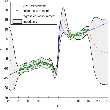
Since purely non-parametric GPR model is data-driven, it lacks interpretability for the system. The another drawback of the model is that when the new test point is far away from the training data, the corresponding output will quickly tend toward zero, as shown in Figure 1. It results high requirement for the training data. Parametric model is use to attempt to represent a particular phenomenon. However, to build these models, substantial domain expertise is required. It results that these accurate parametric models are difficult to obtain, which are always very complicated and are often simplified to represent the actual systems.

-25 -20 -15 -10 -5 0 5 10 15 20 25 -25

-20 -15 -10 -5 0 5 10 15 20 25

x

y

[image:4.612.103.283.481.661.2]

true measurement noise measurement regression measurement uncertainty

Figure 1: Gaussian Process Regression For A One-Dimensional Linear Regression Problem,

t t t t

t x x x w

y = /2+25 /(1+ 2)+ , With w_t ~N(0,1) I.I.D. Noise.

The Blue Line Denotes The Noise-Free Measurements. The Red Dashed Denotes The

Output Of Trained GPR Model Using The Training Data (Green Circle), Which Are Collected In Both Areas [-20, 0] And [5, 15]. The Gray Region Denotes The 95% Confidence Region For Regression Measurements. Note That Both The Error Of Regression Measurement And Its Uncertainty (The Vertical Width Of The Gray Region) Become Larger Beyond The Training Areas.

The combinated model of GPR and parametric models can alleviate some of the problems with either model alone. Since the GPR model is used to represent the aspect of the dynamic system that is still not modeled by the parametric model, the accuracy of the combinated model for the actual system is improved. Meanwhile, due to the parametric model can capture most of the physical process underlying the dynamic system, the generality of the combinated model is improved beyond the training data. The combinated model is called Model-enhanced GP (MEGP) model.

The GPR-model branch of MEGP model is used to represent the residual output after factoring the contribution of the parametric model. If

) ( −1

= k

k f x

x and zk =h(xk) are the parametric state-space models for the dynamic system, then the MEGP model can be written as

) , ( GP )

( 1 1

f f

µ x

x f

xk= k− + k− D

) , ( GP )

(x µh x h

h

zk= k + k D

where GP ( 1, ) f f _x

D

k− and GP ( , ) h h _x

D

k are the GPR-model branches of MEGP models for the transition and measurement models, respectively. The training outputs for the two MEGP models are

) ( −1 − =

∆xk xk f xk ). ( −1 − =

∆zk zk h xk Their corresponding training data are

), , (X0 X

f _{= ∆}

D

) , (X Z

h_{= ∆}

D

where X₀ =[x₀,x₁,_L,x_N−1] , X=[x₁,x₂,_L,x_N],

] , , ,

[ x₁ x₂ x_N

X= ∆ ∆ ∆

∆ _L ,

] , , ,

[ z₁ z₂ z_N

Z= ∆ ∆ ∆

∆ _L .

Now the MEGP models can be incorporated into the SRCKF algorithm. Details of the resulting filtering algorithm are presented in Appendix A.

5 APPLICATIONS

is considered in this paper. This model is highly nonlinear and bimodal that is really challenging for traditional filtering techniques. The dynamic state space model for UNGM can be written as

, )) 1 ( 2 . 1 cos( 8 1

25 2

1

1 2

1 1

1 −

− −

− + ₊ + − +

= _k

k k k

k k w

x x x

x (13)

, , , 2 , 1 ,

20

1 2

K k

v x

y_k = _k+ _k = _L (14)

where w_k−₁~N(0,σ_w2) and vk ~N(0,σv2) . The cosine term in the state transition model represents the effect of time-varying noise.

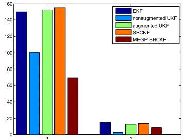
First, we assume that the accurate parametric model is obtained as Eq. (13) and Eq. (14). EKF, nonaugmented UKF, augmented UKF [13], and SRCKF are also tested in this case. In figure 2 we have plotted the mean square errors (MSEs) of each tested methods of 50 Monte Carlo runs, of which the mean and standard deviation is present in figure 3.

0 5 10 15 20 25 30 35 40 45 50

0 50 100 150 200 250 300

[image:5.612.106.284.324.463.2]

EKF nonaugmented UKF augmented UKF SRCKF MEGP-SRCKF

Figure 2: MSEs of different methods in 50 Monte Carlo runs

1 2

0 20 40 60 80 100 120 140

[image:5.612.325.509.348.487.2]

EKF nonaugmented UKF augmented UKF SRCKF MEGP-SRCKF

Figure 3: The Means (Left) And Standard Deviations (Right) Of Mses Of Different Methods In 50 Monte Carlo

Runs

Since the bimodality of UNGM in general can not be applied well using Gaussian approximations, EKF don’t work well in this case. The

MEGP-SRCKF can obtain similar results to the augmented UKF and the SRCKF. They give clearly better performance from the nonaugmented UKF. In the case that we can obtain appropriate parametric models, the MEGP-SRCKF can obtain similar performance to its corresponding parametric filter.

We further assume that an insufficiently accurate state-space model is obtained as follows:

, 1

30 3

1

1 2

1 1

1 −

− −

− +

+ +

= _k

k k k

k w

x x x

x

, 10

1 2 k k

k x v

y = +

Before filtering, two groups data are assumed to obtain for training the GPR-model branch of MEGP models for the transition and measurement models, respectively. We also test the above filters in this case. Similarly, in Figure 4 we have plotted the MSEs of each tested methods of 50 Monte Carlo runs, of which the mean and standard deviation is present in Figure 5.

0 5 10 15 20 25 30 35 40 45 50

50 100 150 200

[image:5.612.106.285.495.630.2]

EKF nonaugmented UKF augmented UKF SRCKF MEGPSRCKF

Figure 4: Mses Of Different Methods In 50 Monte Carlo Runs

1 2

0 20 40 60 80 100 120 140 160

EKF nonaugmented UKF augmented UKF SRCKF MEGP-SRCKF

Figure 5: The Means (Left) And Standard Deviations (Right) Of Mses Of Different Methods In 50 Monte Carlo

[image:5.612.327.505.531.667.2]

As shown in Figure 4 and 5, we can see that the MEGP-SRCKF is effective to estimate the state in this case, whereas standard EKF, nonaugmented UKF, augmented UKF, and SRCKF are disabled. Compare the results of the above four figures, it also shows that MEGP-SRCKF can obtain the similar results whether the accurate parametric state-space model can be obtained. Therefore, the MEGP-SRCKF does not require an accurate, parametric model of the nonlinear dynamic system.

6 CONCLUSIONS

An alternative estimation algorithm called CKF has been proposed recently for nonlinear dynamic systems. It can preserve the first and second moments accurately with low computation. However, its performance relies on the accurate state-space models as same as the traditional filters, for instance EKF and UKF. In this paper, a novel filter algorithm called MEGP-SRCKF is presented to estimate the state of nonlinear dynamic systems where their transition or measurement or both models are unknown or insufficiently accurate. It integrated a combination model of GPR and parametric models into the SRCKF, where the state-space model is replaced by the combination model. The GPR-model branch of the combination model is used to learn and represent the residual aspects of the system that are not captured by the parametric model. The novel algorithm alleviates the disadvantages associated with the traditional filters, and its performance is tested via two examples.

Appendix A: Table 1 Megp-Srckf Algorithm

Before Filtering

1) Build the training data for the transition MEGP model and train this model:

). , ( GP ~ 1 f f _x

xk k− D

∆

2) Build the training data for the measurement MEGP model and train this model:

). , ( GP

~ h x h

z_{k k} D

∆

3) Evaluate the initial cubature points (i=1,2,_L,m, m=2nx)

. ] 1 [ i x

i= n

ξ

Initialization

1) Initialization of the state x0|0 and the square-root factor of the predicted error covariance S0|0 such that

T S S P0|0 = 0|0 0|0.

Time Update

1) Evaluate the cubature points of the current state (i=1,2,_L,m)

1 | 1 1 | 1 1 | 1

,k−k− = k−k− i+ˆk−k−

i S

X ξ x .

2) Evaluate the cubature points of the predicted state (i=1,2,L,m)

) , (

GP )

( , 1| 1 , 1| 1 * 1 | , f f µ

f X X D

Xikk− = ik−k− + ik−k− . 3) Estimate the predicted state

∑

= − − = m i k k i k k X m 1 * 1 | , 1 | 1 ˆ x .

4) Estimate the square-root factor of the predicted error covariance

[

]

(

, 1

)

* 1 | 1 1

|k− = k−k− k−

k S

S Tria X _Q

where the weighted, centered matrix

[

]

1 | * 1 | 1 , 1 | * 1 | 1 , 2 1 | * 1 | 1 , 1 * 1 | 1 ˆ ˆ ˆ 1 − − − − − − − − − − − − − − = k k k k m k k k k k k k k k k X X X m x x x L X

and SQ,k−1 denotes a square-root factor of

) , ˆ (

GP _{1| 1}

1

f f

Σ xk k D

k− = − −

Q such that

T k k k−1=SQ,−1SQ, −1

Q .

Measurement Update

1) Evaluate the cubature points of the update state(i=1,2,_L,m)

1 | 1 | 1 |

,kk− = kk− i+ˆkk−

i S

X ξ x .

2) Evaluate the cubature points of the predicted measurement (i=1,2,_L,m)

) , ( GP )

( _{,| 1 ,| 1}

1 | , h h µ

h X X D

Z_ikk− = _ikk− + _ikk− . 3) Estimate the predicted measurement

∑

= − − = m i k k i k k Z

m ₁ ,| 1 1

|

1 ˆ

z .

4) Estimate the square-root factor of the innovation covariance matrix

[

]

(

kk k

)

k

k S

Szz_,|−1=Tria Z_{| −1 R,}

where the weighted, centered matrix

[

]

1 | 1 | , 1 | 1 | , 2 1 | 1 | , 1 1 | ˆ ˆ ˆ 1 − − − − − − − − − − = k k k k m k k k k k k k k k k Z Z Z m z z z L Z

and SR,k denotes a square-root factor of

) , ˆ (

GP_Σh x_{k|k 1} Dh

k= −

R such that Rk =SR,kSTR,k. 5) Estimate the cross-covariance matrix

T k k k k k k

P_xz,|−1=X_{| −1}Z_|−1

where the weighted, centered matrix

[

]

1 | 1 | , 1 | 1 | , 2 1 | 1 | , 1 1 | ˆ ˆ ˆ 1 − − − − − − − − − − = k k k k m k k k k k k k k k k X X X m x x x L X .

1 | , 1 | , 1 |

, / )/

( _{− − −}

= T _kk

k k k k

k P S S

W _{xz zz zz} .

7) On the receipt of a new measurement zk, estimate the updated state

) ˆ ( ˆ

ˆ_k|k =x_k|k−1+W_k z_k −z_k|k−1

x .

8) Estimate the square-root factor of the update error covariance matrix

[

]

(

kk k kk k k

)

k

k W W S

S _| =Tria X_{| −1}- Z_{|−1 R,} .

REFRENCES:

[1] R. E. Kalman, R. S. Bucy, “New results in linear filtering and prediction theory”, Trans. ASME Ser. D J. Basic Eng., Vol. 83, 1961, pp. 95-108. [2] A. H. Jazwinski, “Stochastic Processes and

Filtering Theory”, New York: Academic Press, 1970.

[3] P. S. Maybeck, “Stochastic Models, Estimation, and Control”, vol. 141 of Mathematics in Science and Engineering, New York: Academic Press, 1979.

[4] S. J. Julier, J. K. Uhlmann, “A new extension of the Kalman filter to nonlinear systems”, Proceedings of AeroSense: 11th Symposium on Aerospace/Defense Sensing, Simulation and Controls, Orlando, FL, USA, 1997, pp. 182-193.

[5] M. Opper, “A Bayesian approach to online learning”, In Online Learning in Neural Networks, Cambridge University Press, 1998, pp. 363-378.

[6] K. Ito, K. Xiong, “Gaussian filters for nonlinear filtering problems,” IEEE Trans. Automatic Control, Vol. 45, No. 5, 2000, pp. 910-927. [7] I. Arasaratnam, S. Haykin, R. J. Elliott,

“Discrete-time nonlinear filtering algorithms using Gauss-Hermite quadrature”, Proc. IEEE, Vol. 95, No. 5, 2007, pp. 953-977.

[8] F. Gustafsson, G. Hendeby, “Some Relations Between Extended and Unscented Kalman Filters,” IEEE Trans. Signal Processing, Vol. 60, No. 2, 2012, pp. 545-555.

[9] I. Arasaratnam, S. Haykin, “Cubature kalman filters”, IEEE Trans. on Automatic Control, Vol. 54, No. 6, 2009, pp. 1254-1269.

[10]J. Ko, D. Fox, “GP-BayesFilters: Bayesian filtering using Gaussian process prediction and observation models”, Autonomous Robots, Vol. 27, No. 1, 2009, pp. 75-90.

[11]F. L. Lewis, “Optimal Estimation”, New York: Wiley, 1986.

[12]C. E. Rasmussen, C. K. I. Williams, “Gaussian Processes for Machine Learning”, MIT Press, 2006.