ASSOCIATION RULE MINING BASED VIDEO CLASSIFIER WITH LATE ACCEPTANCE HILL CLIMBING APPROACH

(1)

ISSN: 1992-8645 www.jatit.org E-ISSN: 1817-3195

NONLINEAR SYSTEM IDENTIFICATION

BASE ON FW-LSSVM

1,2 _{XIANFANG WANG,} 1_{YUANYUAN ZHANG,}1_{JIALE DONG,}3_{ZHIYONG DU}

1_{College of Computer & Information Engineering, Henan Normal University, Xinxiang 453007, China}

2_{Henan Province Colleges and Universities Engineering Technology Research Center}

for Computing Intelligence & Data Mining, Xinxiang 453007, Henan, China

3_{Henan Mechanical and Electrical Engineering College, Xinxiang 453002, Henan, China}

E-mail: [email protected]

ABSTRACT

This paper proposed a method to identify nonlinear systems via the fuzzy weighted least squares support machine (FW-LSSVM). At first, we describe the proposed modeling approach in detail and suggest a fast learning scheme for its training. Because the training sample data of independent variable and dependent variable has a certain error, and we obtain the sample which has a certain fuzziness from measuring, influencing the accuracy of model building, this paper would put the concept of fuzzy membership into the least squares support vector machine. Using the fuzzy weighted least squares algorithm for samples, each sample in the vector is introduced into the fuzzy membership degree, this improve the anti noise ability of least squares support vector machine. The efficiency of the proposed algorithm was demonstrated by some simulation examples.

Keywords: Mixed Kernel Function, FW-LSSVM, Identification，Nonlinear Systems.

1. INTRODUCTION

Most systems encountered in the real world are nonlinear in nature, and since linear models cannot capture the rich dynamic behavior of limit cycles, bifurcations, etc. associated with nonlinear systems, it is imperative to have identification techniques which are specific for nonlinear systems[1-4].

SVM is employed to realize some complex nonlinear desired functions, which is presented by Vapnik and based on the statistical learning theory and learning method has obtained certain achievements. SVM has strong generalization ability in solving the small sample, nonlinear, high dimension, and local minimum of practical problems. SVM use a variety of kernel function which can be classified into global kernel function and local kernel function [5]. Smits and Jordaan use the two kernel function to make up a kind of mixed kernel function through the research on two kinds of representative global kernel function (polynomial kernel function) and local kernel function (RBF kernel function) mapping properties [6]. In addition, Suykens presents a least squares vector machine (LSSVM) method based on SVM. LS-SVM transform the traditional SVM inequality constraints into equality constraints, in order to avoid a quadratic programming problem solving

time-consuming, and LS-SVM reduce the run time, and effectively improve the speed of learning to solve at a large extent. Although the algorithm and the structure of the LS-SVM are simple, and the calculation of LS-SVM is fast, it lost the loose and robustness of SVM in a certain extent.

This paper overcome the adverse effects of the training sample noise by selecting the fuzzy weighted least squares support vector machine algorithm and putting fuzzy weighted membership on the squared error of each sample [7-9]. Selecting LS-SVM which is constructed with mixed kernel function not only has a good learning ability but also has better generalization ability. Simulation results show that the fuzzy weighted least squares support vector machines help to improve the robustness of the model and have a certain practicality.

(2)

2. THEORY OF LSSVM

LSSVM(Least squares support vector machine）

[5] flow the principle of the structural risk minimization of the SVM algorithm in training process, and the inequality constraints of the objective function in SVM is transformed into the equality constraint. Select a nonlinear mapping and input vector is mapped from the original space to a high dimensional feature space. And the optimal decision function is constructed by using the principle of the structural risk minimization in the high dimensional feature space. Dot product operation in high-dimensional feature space is replaced by the kernel function of the original space, and the first power of the empirical risk is replaced by the square in this procedure. The insensitive loss function is avoided, and the complexity is greatly reduced and that the obtained external solution which is a global optimal solution is ensured.

The article assumes that the sample training set is given. The sample training set is

{

x y x y x y

}

Rn R

l

l, ) ∈ ×

( ) , ( ), ,

( 1 1 2 2 L , and xl is

the l th− sample of the input mode and

y

_l is the

l th− the desired output of the l th− sample, and l is the total number for the training sample. The samples are mapped to the high-dimensional feature space from the original space _{R by using the}n nonlinear mappingϕ ⋅

( )

. In the feature space, the

model of least square support vector machine is

( ) T ( )

y x =w ϕ x +b (1)

where ϕ( )x is the feature mapping and

w

T

represents the weight vector, and b is the offset vector.

Based on the structural risk minimization the recursive model of LS-SVM for solving the function (1) is

)

(

2 1 1 min , 2 2 l T i i

J w e w w

=

γ

= +

∑

ξ (2)

.

.t

s

y

_i

=

w

T

ϕ

(

x

_i

)

+

b

+

ξ

_i

where γ is called the adjustable constant and

0

γ > ,

ξ

_i is the error term, andξ ≥_i 0.

The corresponding Lagrangian function for (2) is as follows

{

}

2 2 1 1 1 ( , , , ) 2 2 ( ) l i i l T

i i i i

i

L w b w

w x b y

=

γ

ξ α = + ξ −

α ϕ + + ξ −

∑

(3)

where α_i is Lagrange multiplier and

[

1, 2 ,

]

T l

α = α α L α . Based on KKT which is the optimal conditions, the linear equations are obtained after eliminate ξ_iandw .

1

0 ( )

0 0

0

0 ( )

l i i i l i i

i i i

T

i i i

L w x w L b L L

y w x b

=

∂ 

= → = α ϕ

 _∂ 

 _{∂ = → α =}

 _∂ 

∂

 _{= → α = γ ξ}

 _∂ξ

 ∂

 _{= → =} _ϕ _{+ + ξ}

_∂α 

∑

(4)

Then the optimization problem is transformed into the following linear equation:

1 1 1 1

1 1

0 1 1

0 1

1 ( , ) ( , )

1

1 ( , )_l _l ( , )_l _l l l

b

K x x K x x _y

y

K x x K x x

 

   

 

   

+

 _γ _α

   

  ₌

   

 

   

 _α

+    

 _γ

 

L

M M

M M L M

L

(5)

where ( , ) ( )T ( )

k l k l

K x x = ϕ x ϕ x is the kernel function . Linear kernel, polynomial kernel and RBF kernel are the common kernel functions. In this paper, the mixture kernels which consist of polynomial kernel and RBF kernel are used. The expression is as follow

2

2 2

[( ) 1] (1 ) exp( / )

mix i i

K = ρ ⋅x x + + −ρ − −x x σ

(6)

whereρ( 0≤ ρ ≤1) is the constant to regulate the

effect of the two kernel functions. It is important to select the parameters ρ σ, and the

penalty-factorC . In order to get the model that has the predicted effect, it is necessary to optimize and adjust the parameters [10-11].

3. FW- LSSVM

(3)

2 1

1 min ( , )

2 2

l T

i i i

J w e w w e

=

γ

= +

∑

µ (7)

The corresponding Lagrangian function for Equation (7) is as follows:

{

}

2 2 1 1 1 ( , , , ) 2 2 ( ) l i i i l T

i i i i

i

L w b w

w x b y

=

γ

ξ α = + µ ξ −

α ϕ + + ξ −

∑

(8)

The linear equations are obtained for the function (8):

1

0 ( )

0 0

0

0 ( )

l i i i l i i

i i i i

T

i i i

L w x w L b L L

y w x b

=

= ∂



= → = α ϕ

 _∂ 

 _{∂ = → α =}

 ∂



∂

 _{= → α = γ µ ξ}

 _∂ξ 

∂

 _{= →} ₌ _ϕ _{+ + ξ}

_∂α 

∑

(9)

Then the optimization problem of the function (9) is transformed into the following linear equation:

1 1 1 1

1 1

0 1 1

0 1

1 ( , ) ( , )

1

1 ( , ) ( , )

i

l l

l l l l

i

b

K x x K x x _y

y

K x x K x x

 

   

 

+    

 _γµ  _α

      ₌             α +    

 _γµ

 

L

M M

M M L M

L

(10)

The parameters αand b can be obtained by the Equation(10), and selecting the weighted coefficient µ_i is based on the error ξ = α γ_i _i/ of the LS-SVM.

4. IDENTIFICATION VIA FW-LSSVM

Consider the nonlinear system

( ) ( ( 1), ( 1) , , ( ) ,

( 1) , ( 2 ) , , ( ))

y k f y k y k y k n

u k u k u k m

= − − −

− − −

L

(11)

where u(k) is the system input, y(k) the system output; where m and n are respectively the delays of u(k) and y(k). f(.) is a nonlinear function.

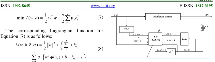
The identification of nonlinear system based on FW-LSSVM model is depicted in Figure 1.

( ) ( ( 1), ( 1) , , ( ) ,

( 1) , ( 2 ), , ( ) )

M s v m M M M

y k f y k y k y k n

u k u k u k m

= − − −

− − −

L

(12)

where y_M( )k is the output of the identification model,

( )

S V M

f g is the obtained model by training FW-LSSVM.

Nonlinear system

FW-LSSVM TDL TDL

u(k-1 )

u(k-m+1)

+ ym(k-1)

Z-1

ym(k+1 )

ym(k-n+1)

ym(k)

y(k)

_ u(k)

e(k)

[image:3.612.89.526.70.196.2]

. . . . . .

Figure 1: The Diagram Identification Of The Nonlinear System Based On SVR

The detailed process of this identification can be described as following:

Step 1 Chose the input signal u(t) for the nonlinear system Equation(11).

Step 2 Chose the sampling time t , sampling _s

dots N and width of window is t=N t* _s.

Step 3 Initialed the input and output, and obtained the values of u(k) and output y(k) at every sampling time k .

Step 4 Choose the delays of input m and output n

(m≥ ≥n 0). Construct a sampling set D={ , }X Y , where

( ) { ( 1), ( 2), , ( ),

( 1), ( 2), , ( )}

( ) ( )

( 1), ,

X k m y k y k y k n

u k u k u k m

Y k m y k

k m N

− = − − −   − − −   − =   ₌ ₊  L L L

Step 5 Chose the kernel function K x x( ,_i _j) determine parameters of the FW-LSSVM (such asγ µ, _i)

Step 6 Computing the output Y_M when the input is, and the training error E= −Y Y_M.

Step 7 If the error E is less than a threshold ,the training is over, then go to the next step; else return to Step 5.

Step 8 The parameter vector wwould be obtained

by solving quadratic regulation in Equation (9) .

Step 9 The model is obtained , the identification

process of nonlinear system is end.

5. THE SIMULATION EXPERIMENT

(4)

computer and the software of Matlab 7.0 are needed to accomplish the experiment.

The nonlinear model is as follow [13]: ( 1) 0.6 * ( ) /(1 ( ) * ( ))

0.3* ( ) * ( ) 0.8 * ( )

y k y k y k y k

u k y k u k

+ = +

+ + (13)

The data need to be trained before test the fuzzy weighted least squares support vector machine. The input sample of the training data are structured the array and every row of the array represents the input vector. The training sample is:

( ) [ ( 2 ) , ( 1) ,

( 2 ), ( 1) , ( ) ]

( ) ( 3)

X k y k y k

u k u k u k

Y k y k

= + +

 

+ +



 ₌ ₊



(14)

In the model, the sampling time t_s =0.01s ,

sampling dots N =200 , the width of window is .t=N t* _s =2s. The mixture kernel function

2

2 2

[( ) 1] (1 ) exp( / )

mix i i

K = ρ x x⋅ + + − ρ − −x x σ is used.

The parameters of the kernel function has the stronger influence, so the value of ρ is 0.01 through the experience. The output of the training data in the model are compared with the actual output until the error is the minimum. The vectors of σ and γ are gained when the error is the

[image:4.612.304.528.77.235.2]

minimum. The vector of σ is 0.2756 and the positive number γ is 200. Figure 2 is the output of the simulated nonlinear system model and the Figure 3 is the output error of modeling.

0 0.2 0.4 0.6 0.8 1 1.2 1.4 1.6 1.8 2 0

0.5 1 1.5 2 2.5 3 3.5

t/s

y

o

u

t

Figure 2: The Output Of The Training Model

0 0.2 0.4 0.6 0.8 1 1.2 1.4 1.6 1.8 2 -0.015

-0.01 -0.005 0 0.005 0.01 0.015 0.02 0.025 0.03 0.035

[image:4.612.318.523.384.534.2]

t/s e1

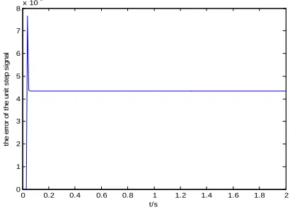
Figure 3: The Training Error Curve Of When The Input Is A Random Signal

In the fuzzy weighted least squares support vector machine of the nonlinear system, the random signal u kr( )=rand(1) , unit step signal, sinusoidal

signal 0.5 sin(2π +t 0.5) and the square signal

0.5sign(sin(2 )) 0.5π +t are used to test the

generalization performance of the model. The output error curves of the fuzzy weighted LS-SVM nonlinear system identification model are the figure from Figure 4 to Figure 6.

0 0.2 0.4 0.6 0.8 1 1.2 1.4 1.6 1.8 2 0

1 2 3 4 5 6 7 8x 10

-3

t/s

th

e

rr

o

r

o

f

th

e

u

n

it

s

te

p

s

ig

n

a

l

Figure 4: The Identification Error Curve When

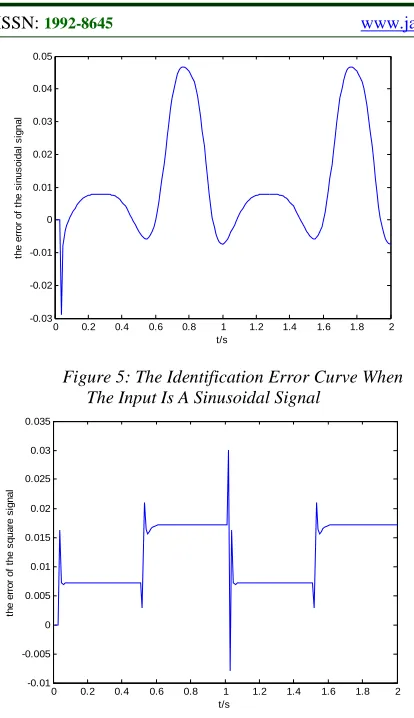
[image:4.612.93.295.446.576.2]

(5)

0 0.2 0.4 0.6 0.8 1 1.2 1.4 1.6 1.8 2 -0.03

-0.02 -0.01 0 0.01 0.02 0.03 0.04 0.05

t/s

th

e

rr

o

r

o

f

th

e

s

in

u

s

o

id

a

l

s

ig

n

a

l

Figure 5: The Identification Error Curve When The Input Is A Sinusoidal Signal

0 0.2 0.4 0.6 0.8 1 1.2 1.4 1.6 1.8 2 -0.01

-0.005 0 0.005 0.01 0.015 0.02 0.025 0.03 0.035

t/s

th

e

rr

o

r

o

f

th

e

s

q

u

a

re

s

ig

n

a

[image:5.612.93.300.70.429.2]

l

Figure 6: The Identification Error Curve When The Input Is A Square Signal

Figure 3 to Figure 6 indicate that using the fuzzy weighted LS-SVM avoids the over-fitting reduces the incompactness. The simulation experiment proves that the fuzzy weighted LS-SVM nonlinear system has a better robust.

6. CONCLUSIONS

In this paper, we present an improvement method to identify nonlinear system. The algorithm is put the fuzzy weighted to use LSSVM. Based on that the samples have different and important influence in every model of the productive process, fuzzy weighted algorithm is introduced. The influence of the abnormal training data are overcame and the over-fitting of the identification model is avoided. The simulation experiment indicates that the fuzzy weighted LS-SVM and the mixture kernel function avoids the algorithm convergent prematurely and improves the fuzzy learning precision and the generalization ability. Then the robustness of the system is improved and the fuzzy weighted LS-SVM has a better

application. The results demonstrate that the suggested method gives better error minimization for nonlinear system.

ACKNOWLEDGEMENTS

This work is supported by the National Natural Science Foundation of China (No.61173071), the Science and Technology Research Project of Henan Province(No.122102210079), the Foundation and Frontier Technology Research Programs of Henan Province(No.112400430087), the Innovation Talent Support Program of Henan Province Universities (No.2012HASTIT011), the Doctoral Started Project of Henan Normal University(No.1039)

REFERENCES:

[1] Musa Alci, Musa H. Asyali, “Nonlinear system identification via Laguerre network based fuzzy systems”, Fuzzy Sets and Systems, Vol. 160, No. 24, 2009, pp. 3518-3529.

[2] Johan Paduart, Lieve Lauwers, Jan Swevers, Kris Smolders, Johan Schoukens, Rik Pintelon, “Identification of nonlinear systems using Polynomial Nonlinear State Space models”, Automatica, Volume 46, No. 4, 2010, pp. 647-656.

[3] Alireza Rahrooh, Scott Shepard, “Identification of nonlinear systems using NARMAX model ”, Nonlinear Analysis: Theory, Methods & Applications, Vol. 71, No. 12, 2009, pp. e1198-e1202.

[4] Gregor Dolanc, Stanko Strmčnik, “Identification of nonlinear systems using a piecewise-linear Hammerstein model”, Systems & Control Letters, Vol. 54, No. 2, 2005, pp. 145-158.

[5] Suykens J A K, ‘“Vandewalle J. Least squares support vector machine classifiers”, Neural Processing Letters, Vol. 9, No. 3, 1999, pp. 293-300.

[6] Mao Zhi-liang, Liu Chun-bo, Pan Feng, “Parameter Selection and Application of SVM with Mixture Kernels Based on IPSO”, Journal of Southern Yangtze University, Vol. 8, No. 6, 2009,

pp.

632-634.

[7] Zhang Ying, Su Hong-ye, Chu Jian, “Soft sensor modeling based on fuzzy least squares support vector machines”, Control and

Decision, Vol. 20, No. 6, 2005, pp.621-624.

(6)

Making Information Based on Fuzzy Weighted Least Squares Method”, Journal of Shang Hai Jiao Tong University. Vol. 43, No. 9, 2009,

pp.

1377-1382.

[9] Li Zheng, Song Bao-wei, Mao Shao-yong, “Fuzzy Weighted Linear Regression on Zero Failure Exponent Distribution”, Journal of System Simulation, Vol. 17, No. 6, 2005,

pp.

1373-1375.

[10] Xiong Wei-li, Wang Xiao, Chen Min-fang, Xu Bao-guo, “Modeling for penicillin fermentation process based on weighted LS-SVM”, CIESC Journal, Vol. 63, No. 9, 2012,

pp.

2913-2918

[11] Wu Tie-bin, Liu Yun-lian, Li Xin-jun, Yin Yong-sheng, “KPCA-fuzzy Weighted LSSVM Based Prediction Method and its Application”, Computer Measurement and Control, Vol. 20, No. 3, 2012,

pp.

617-620.

[12] Guo Hui, Liu He-ping, Wang Ling. “Method for Selecting Parameters of Least Squares Support Vector Machines and Application”, Journal of System Simulation, Vol. 18, No. 7, 2006,

pp.

2033-2036.