Option pricing under the double
exponential jump diffusion model with
‐
stochastic volatility and interest rate
Chen, R, Li, Z, Zeng, L, Yu, L, Qi, L and Liu, JL
http://dx.doi.org/10.3724/SP.J.1383.204012
Title
Option pricing under the double exponential jump diffusion model with
‐
stochastic volatility and interest rate
Authors
Chen, R, Li, Z, Zeng, L, Yu, L, Qi, L and Liu, JL
Type
Article
URL
This version is available at: http://usir.salford.ac.uk/44888/
Published Date
2017
USIR is a digital collection of the research output of the University of Salford. Where copyright
permits, full text material held in the repository is made freely available online and can be read,
downloaded and copied for noncommercial private study or research purposes. Please check the
manuscript for any further copyright restrictions.
For more information, including our policy and submission procedure, please
contact the Repository Team at:
.
Stochastic Volatility and Interest Rate
Chen Rongda, Li Zexi, Zeng Liyuan, Yu Lean, Qi Lin and Liu Jia
Citation: Journal of Management Science and Engineering 2, 252 (2017 ); doi: 10.3724/SP.J.1383.204012 View online: http://engine.scichina.com/doi/10.3724/SP.J.1383.204012
View Table of Contents:http://engine.scichina.com/publisher/CSPM/journal/JMSE/2/4 Published by the Science Press
Articles you may be interested in
Pricing vulnerable European options under a two-sided jump model via Laplace transforms SCIENTIA SINICA Mathematica 45, 195 (2015);
Pricing Continuously Monitored Barrier Options under the SABR Model: A Closed-Form Approximation
Journal of Management Science and Engineering 2, 116 (2017);
A Binomial Model of Asset and Option Pricing with Heterogeneous Beliefs Journal of Management Science and Engineering 1, 94 (2016);
Valuation of equity-indexed annuities with regime-switching jump diffusion risk and stochastic mortality risk
SCIENCE CHINA Mathematics 55, 2335 (2012);
Indifference pricing and hedging in a multiple-priors model with trading constraints SCIENCE CHINA Mathematics 58, 689 (2015);
doi:10.3724/SP.J.1383.204012 http://engine.scichina.com/publisher/CSPM/journal/JMSE
Article
Option
Pricing
under
the
Double
Exponential
Jump
‐
Diffusion
Model
with
Stochastic
Volatility
and
Interest
Rate
Rongda
Chen
1, 2
,
Zexi
Li
1, 3,
Liyuan
Zeng
4
,
Lean
Yu
5,
*,
Qi
Lin
1
and
Jia
Liu
6
1 School of Finance, Zhejiang University of Finance and Economics, Hangzhou 310018, China; [email protected];
2 Collaborative Innovation Center for Wealth Management and Quantitative Investment, Zhejiang University of Finance and
Economics, Hangzhou 310018, China
3 School of Economics and Management, University of Chinese Academy of Sciences, Beijing 100190, China; [email protected]
4 PricewaterhouseCoopers Zhong Tian LLP, Beijing Branch, Beijing 100020, China; [email protected]
5 School of Economics and Management, Beijing University of Chemical Technology, Beijing 100029, China
6 Salford Business School, Salford University, Salford M5 4WTU, UK; [email protected] * Correspondence: [email protected]
Received: 26 July 2017; Accepted: 3 December 2017; Published: 21 December 2017
Abstract: This paper proposes an efficient option pricing model that incorporates stochastic interest rate (SIR),
stochastic volatility (SV), and double exponential jump into the jump‐diffusion settings. The model
comprehensively considers the leptokurtosis and heteroscedasticity of the underlying asset’s returns, rare events,
and an SIR. Using the model, we deduce the pricing characteristic function and pricing formula of a European
option. Then, we develop the Markov chain Monte Carlo method with latent variable to solve the problem of
parameter estimation under the double exponential jump‐diffusion model with SIR and SV. For verification
purposes, we conduct time efficiency analysis, goodness of fit analysis, and jump/drift term analysis of the proposed
model. In addition, we compare the pricing accuracy of the proposed model with those of the Black–Scholes and the
Kou (2002) models. The empirical results show that the proposed option pricing model has high time efficiency, and
the goodness of fit and pricing accuracy are significantly higher than those of the other two models.
Keywords: Option pricing model; Stochastic interest rate; Stochastic volatility; Double exponential jump; Markov
Chain Monte Carlo with Latent Variable
1. Introduction
In the last decade, many studies have examined the pricing of financial securities using the various jump‐diffusion
Cheng and Scaillet, 2007; Wong and Lo, 2009; Kim and Kim, 2011; Chiarell and Kang, 2013; Kim et al., 2014; Wang et al.,
2016; Kiesel and Rahe, 2017; Leippold and Schärer, 2017). In addition, research departments in the financial industry have
begun using jump‐diffusion models as an evaluation tool (Zhang and Wang, 2013). This increase in interest is due largely
to the following reasons. First, jump‐diffusion models can partly explain the leptokurtic features of the distribution of the
asset returns, which may have a higher peak and heavier tails than in the case of the normal distribution. Second, these
models can deal effectively with other empirical phenomena, such as the volatility smiles in option markets. As a result,
they are used to model both the overreaction (attributed to heavy tails) and the under‐reaction (attributed to high peaks)
to external good or bad news in financial markets (Barndorff‐Nielsen and Shephard, 2006; Maekawa et al., 2008). Thus,
the jump component of the jump‐diffusion settings can be viewed as the financial marketʹs response to signals provided
by external events.
The two prominent normal jump‐diffusion models (Merton, 1976) and the double exponential jump‐diffusion
model (Kou, 2002) can all partly interpret the leptokurtic features of a distribution and the volatility smile. As a
result, many studies have employed normal jump‐diffusion settings in an attempt to explain two empirical
phenomena: normal jump‐diffusion models utilizing a stochastic interest rate (SIR), and the stochastic volatility (SV)
of Glasserman and Kou (2003), Johannes (2004), Espinosa and Vives (2006), Bo et al. (2010), Beliaeva and Nawalkha
(2012), Pillay and O’Hara (2011), and Simonato (2011).
Empirical studies have indicated that the double exponential jump‐diffusion model fits the asset price process
better than the normal jump‐diffusion model does (Ramezani and Zeng, 1998; Barndorff‐Nielsen and Shephard,
2006; Maekawa et al., 2008), which has seen the double exponential jump‐diffusion model gaining the wider
acceptance of the two. As a result, researchers have begun developing more general models by integrating a SIR or
SV into the double exponential jump‐diffusion models. Here, examples include the works of Zhang et al. (2012),
Zhang and Wang (2013), Huang et al. (2014), and Leippold and Vasiljevi´c (2017).
However, some models that have been constructed to determine option prices do not simultaneously
incorporate an SIR, SV, and double exponential jumps and, therefore, do not fully capture the leptokurtic features of
asset returns or the volatility smile in option markets. For example, these models have been unable to capture
volatility clustering and the heteroscedasticity effect. Furthermore, the spot interest rate is a fundamental economic
variable in the asset price process, and so cannot be treated as a constant. Zhang and Wang (2013) proposed an
option pricing model that does integrate an SIR, SV, and double exponential jumps. However, their pricing formula
is limited to determining the price of a European option, and so cannot be generalized to other financial derivatives.
In addition, a typical shortcoming of these previous studies is that most focus on numerical computations using
hypothesized parameters. In other words, the parameters are not estimated from real data. Incorporating an SIR, SV,
and jumps simultaneously increases the complexity of estimating the parameters. The maximum likelihood
estimation method cannot be applied in this case, because it is very difficult to obtain the probability density
function of the jump‐diffusion model (Li et al., 2016). In addition, the moment estimation method cannot be used
because the models’ high‐order moments have many parameters and are extremely complex. Another method use
for parameter estimation is the Markov chain Monte Carlo (MCMC) method, which constructs a Markov chain
from the parameter samples (Geman and Geman, 1984; Martino et al., 2015; Meyer et al., 2008; Gilks et al., 1995).
Then, a stable distribution of the parameters is obtained from the chain. The MCMC method has strong adaptability,
which can be used as the basis for estimating the parameters of jump‐diffusion models.
However, when estimating the parameters of the double exponential jump‐diffusion model, there are
(2001) proposed an effective method for dealing with latent variables in the MCMC model. Hu et al. (2006) and Zhou
et al. (2013) proposed using an MCMC estimation for the double exponential jump‐diffusion model, but they
assume that the interest rate and volatility are constant. Then, Yu et al. (2011) proposed using the MCMC method
for the Lévy jump model. Integrating the ideas of these propositions, this paper proposes a method that uses the
Markov chain Monte Carlo model with latent variable (MCMC‐LV) to solve the problem of the parameters in the
jump‐diffusion model making it difficult to estimate.
In addition, we propose several other models that can explain the leptokurtic features and the volatility smile in
option pricing. For example, Chen et al. (2016) proposed American option pricing under generalized mixed
fractional Brown motion (GMFBM), using numerical methods to solve the linear complementarity problem.
However, the parameters of the model are difficult to estimate, and the SIR risk and credit risk cannot be included
in the model. In addition to fractional Brownian motion, the Lévy process is one of the most popular topics among
researchers. Kleinert and Korbel (2016) pointed out that the Lévy process can produce infinite jumps and infinite
variance and, hence, is considered an ideal method to describe heteroscedasticity and rare events (jumps). Fajardo
and Farias (2010) price options by applying the hyperbolic distribution function proposed by Barndorff‐Nielsen
(1977), and assuming that the underlying asset return obeys the Lévy process generated by a multidimensional
generalized hyperbolic distribution. Gong and Zhuang (2016) price options using the underlying asset price process
that contains Lévy volatility and Lévy jump processes. However, the constrained nonlinear optimization method
used by these models lacks stability in the estimated parameters.
In summary, there is still a need for a pricing model that simultaneously incorporates an SIR, SV, and double
exponential jumps, with an effective parameter estimation method for the asset price process. Therefore, we
propose such a model under the affine jump diffusion structure (AJD). It is assumed that SV and the SIR obey the
Cox–Ingersoll–Ross (CIR) process, and that the jump of the underlying asset price follows a double exponential
jump. Our model can incorporate credit risk and expand along multiple dimensions.
The remainder of the paper is organized as follows. In Section 2, we derive the pricing characteristic function
and obtain the pricing formula of a generalized European option, under which a pricing function suitable for the
quick and accurate valuation of European options can be obtained. In Section 3, we propose the MCMC‐LV method
to estimate the parameters in the jump‐diffusion model, taking into account SV and an SIR. In Section 4, we first
verify the effectiveness of the proposed model using a time efficiency analysis, goodness of fit analysis, and
jump/drift term analysis. Then, we compare the pricing accuracy of the proposed model with those of the Black– Scholes (BS) and Kou (2002) models (alternative double exponential jump‐diffusion option pricing models) and the
real market price (10 50ETF European options expiring in June 2016 on the Shanghai Stock Exchange (SSE),
including five call options and five put options with different strike prices). Section 5 concludes the paper.
2. Option Pricing Model under Double Exponential Jump‐Diffusion Settings, with SV and SIR
2.1. Double Exponential Jump‐Diffusion Process, with SV and SIR
In probability space ( , ,ℙ), is the filtration generated by the Brownian motion and the jump process at
time t, 0 t T, and ℙ is a real probability measure. Suppose the instantaneous interest rate r t( ) and the SV
( )t
of the underlying asset of returns are governed by the following CIR process. The basic state process X t( )
(i.e., the underlying asset price S t( )eX t( )) at time
1 ( ) ( ) ( ) ( ) ( ) ( ) ( ) ( ) ( ) 0 0 ( ) ( ( )) 0 ( ) 0 ( ) 0 ( ) ( ) 0 0 ( ) ( ) 0 t t r r r X t d r t d t u t dt t dW t F dJ t t t u W t r r t dt r t d W t dJ t t t W t , (1)where u is the constant drift rate; t follows a double exponential distribution at time t; SV ( )t follows a CIR process; the mean‐reverting rate , long‐term volatility , and volatility of the volatility are constant,
the interest rate r t( ) follows a CIR process; and the mean‐reverting rate r, long‐term mean r , and variation coefficient rare constants. Then, J t( ) is a Poisson process with intensity , and W t W t W t1( ), ( ), r( ), and J t( ) are mutually independent Brownian motions. Moreover, t has an asymmetric double exponential distribution, with density 1 2 1 { 0} 2 { 0} 1 2 ( ) 1 1 ,( 1, 0) f p e q e , in other words, , , d with probability p with probability q , where
and are exponential random variables
with means 1 /1 and 1/2 , respectively, the notation
d
means “equal in distribution,” p0, q0 ,
1
p q , and ,
denote the probabilities of upward and downward jumps, respectively. In addition, the
drift term u
( )t
, and the volatility term
( )t
are assumed to depend affinely on( )t ; that is, these terms attime t are given by
0 1 2 0 2 2 0 0 1 0 1 2 0 0 0 ( ) 0 0 ( ) ( ) 0 0 ( ) 0 0 ( ) ( ) 0 ( ) 0 ( ) 0 0 ( ) 0 0 0 0 0 1 0 0 0 0 , 0 0 , ( ) ( ), 0, 1 0 0 0 0 0 0 r r T r M T M r u u t r t U U t t t t r t t t r t t .At this point, we depict three processes: the basic state process, volatility process, and interest rate process. Let
the price of the underlying asset S t( )eX t( ) be as mentioned above. Then, we have
( ) ( ) ( ) ( ) ( ) 1 1 ( ) ( ) ( ) ( ) ( ) 2 1 ( ) ( )( ( )) ( ) ( ) ( ) ( )( 1) ( ) 2 t t X t X t X t c X t c c X t d e e dX t e dX t dX t e e dJ t dS t S t u t dt S t t dW t S t e dJ t . Let t, 1 t t t V e Y V . Then, we obtain
1 1 ( ) ( )( ( )) ( ) ( ) ( ) ( ) ( ) 2 ( ) ( ) ( ) ( ) ( ) ( ( )) ( ) ( ) t r r r dS t S t u t dt S t t dW t S t Y dJ t d t t dt t dW t dr t r r t dt r t dW t . (2)In order to demonstrate these processes from a clear perspective, the number of underlying assets is assumed
to be one, and the default risk and the correlations between W t W t W t J t1( ), ( ), r( ), ( ),t are ignored. In the following sections, we begin by using Equations (1) and (2) to obtain the pricing characteristic function ( , ( ), , ) t t T of
financial derivatives.
2.2. Double Exponential Jump‐Diffusion Process with SV and SIR under the Risk Neutral Probability Measure
To get the pricing formula for financial securities, it is necessary to carry out a measure transformation for the
double exponential jump process with SV and SIR under the risk neutral probability measure. In this section,
Equations (1) and (2) are transformed under the risk neutral probability measure ℙ. Equations (1) and (2) show that
a double exponential jump process Y dJ tt ( ) cannot be ignored in the process of transforming the measure. Let ( )
1( ), ( ), ( )
T r
W t W t W t W t be a three‐dimensional Brownian motion under real probability measure ℙ,
and ( ) 1 ( ) J t i i Q t Y
be a compound Poisson process with intensity ( +) and jump amplitude Y1, ,Y2 thatfollows the probability density function f y( ) under the real probability measure ℙ . In addition,
1 2 3
( ) ( ), ( ), ( ) T
t t t t
is a three‐dimensional adapted process under the real probability measure ℙ, where
1 3 2 2 1 ( ) i ( ) i t t
.According to theorems on measure transformations of compound Poisson processes and Brownian motions,
the Radon–Nikodym derivative can be obtained as follows:
2 0 0 1 2 1 2 1 ( ) ( ) ( ) ( ) ( ) 2 1 2 1 ( )= ( ), ( ) = ( ) ( ) ( ) ( ) , ( ) ( ) t t T J t u dW u u du t i i i d Z t Z Z t Z t Z t Z t d f Y Z t e Z t e f Y
,where
Z t1( ) is the Radon–Nikodym derivative under the affine process, Z t2( ) is the Radon–Nikodym derivative
under the jump process, Z t( ) is the Radon–Nikodym derivative of the joint measure transformation under both
the affine and the jump process.
Then, under the risk‐neutral probability measure ℙ, the basic state process X t( ), interest rate process r t( ),
and volatility process ( )t at time t are given by:
( ) ( ) ( ) ( ) ( ) ( ) ( ) ( ) t X t d r t d t u t dt t dW t F dJ t t ,where
0 1 2 0 2 2 0 1 1 2 1 0 1 2 ( ) 0 0 ( ) ( ) 0 0 ( ) 0 0 ( ) ( ) 0 ( ) 0 ( ) 0 0 ( ) 0 0 0 0 0 1 0 0 0 0 , 0 0 , ( ) ( ), 1 0 0 0 0 0 0 r r T r M T M r Y u t r t U U t t t t r t t t r t t . (3)Equation (3) is the no‐arbitrage formula of Equations (1) and (2) under the risk neutral probability measure ℙ,
which is the formula of the double exponential jump‐diffusion process with SV and SIR for the underlying asset
price process under the risk‐neutral probability measure. Then, ( )
1( ), ( ), ( )
T r
W t W t W t W t is a three‐dimensional
Brownian motion under the risk‐neutral probability measure ℙ.
2.3. Characteristic Function of Underlying Asset and its Option Pricing Formula
In order to apply the double exponential jump‐diffusion process models with SV and SIR to broaden the range
of financial derivative pricing problems, a generalized pricing formula is required for most of the financial
derivatives in the market.
From Equation (3), the characteristic coefficient of the double exponential jump‐diffusion process model with
SV and SIR is
U U0, , ,1 0 M,1
. Because ( )t is Markovian, decides the following characteristicfunction of the underlying asset (financial derivatives): ( , ( ), , )t t T ( ) ( ) T T t r s ds T e e | ( )t , where 1 3 2 3 .
The characteristic function ( , ( ), , ) t t T denotes the value of an underlying asset at time t that pays
( )
T T
e at future time T , based on all information up to t. The characteristic function ( , ( ), , ) t t T is an
effective tool for pricing options and a wide class of financial derivatives. To solve the characteristic function, the
Feynman–Kac Theorem needs to be used with the double exponential jump model with SV and SIR.
In order to solve the characteristic function, we assume that the characteristic function ( , ( ), , ) t t T has a
solution of the following form, as per Shreve (2004):
( , ( ), , ) exp ( , , ) ( , , )T ( ) t t T t T t T t , where 1 2 3 ( , , ) ( , , ) ( , , ) ( , , ) t T t T t T t T .1 1 2 2 2 1 1 3 2 2 1 1 2 2 1 1 3 2 2 2 2 1 2 2 1 2 2 1 2 ( , , ) ( 1) ( ) tan arctan ( 1) 2 ( 1) ( , , ) 2 ( 1) ( ) tan arctan 2 ( 1 2 2 ( 1) ( , , ) r r r r r r r t T T t t T T t t T 2 2 2 2 2 1 1 2 2 2 1 1 1 2 2 2 2 2 1 1 2 2 2 1 2 1 2 ) ( , , ) ( ) ( ) ( ) 2 ( 1) ( ) 2 ( 1) ( ) 2 ln cos sin 2 2 2 ( 1) ( 2 ln cos r r r r r r r r r r r r r r r r q p r t T Y t T t T t T T t T t r 2 2 2 2 1 1 1 3 2 2 1 1 1) ( ) ( 1) ( ) sin 2 2 ( 1) T t T t . (5)
Equation (5) determines an analytic expression for ( , ( ), , )t t T . For some simple underlying assets with
due payments, ( , ( ), , ) t t T can be used directly. However, for derivative securities such as European options,
the inverse Fourier transform should be applied to the characteristic function ( , ( ), , )t t T .
Next, we derive a European option pricing formula under the double exponential jump model with SV and SIR,
based on the characteristic function ( , ( ), , ) t t T .
Let the price of a generalized European option be ( , , , ( ), , ) C c t t T
( ) ( ) ( ) ln( )1
T T t T r s ds T T ce
e
c
| ( )t , where 1 3 2 3 , 1 3 2 3 (i.e., when T ( ) ln( ) T c is satisfied), and the option pays T ( )T e c at
time T , and zero otherwise. Then, c is a constant, and ln( )c is a threshold, similar to the strike price of a call
option. Let G( , , , ( ), , ) y t t T ( ) ( ) 1 ( ) T T t T r s ds T T y
e e | ( )t be the price of a derivative security at time t.
Then, this derivative security pays T ( )T
e at time T when T ( )
T y
, and zero otherwise. Thus, the pricing
formula of the generalized European option can be written as: C( , , , ( ), , ) c t t T G( , , ln( ), ( ), , )c t t T
(0, , ln( ), ( ), , )
c G c t t T .
From Fubini’s theorem, we define the probability measure ℙ on filtration ( )t , and define the Lebesgue
measure on the real number axis using Borel ‐algebra as ‐addable and complete. Therefore, the order of the
( , , , ( ), , ) ( , , , ( ), , ) y G y t t T G y t t T y
( ) ( )( )
T T t r s ds T Te
e
y
T
|( )
t
,
where G y( , , , ( ), , )y t t T is the partial derivative of G( , , , ( ), , ) y t t T ony. According to the definition,
( , , , ( ), , )
y
G yt t T is absolutely integrable on real number y; thus, G y( , , , ( ), , )y t t T L1[ , ]
.
Therefore, the Fourier transform and inverse Fourier transform of G y( , , , ( ), , )y t t T
exist. Similarly, the
Fourier–Stieltjes transform and inverse Fourier–Stieltjes transform of G( , , , ( ), , ) y t t T exist. The Fourier– Stieltjes transform of G( , , , ( ), , ) y t t T is defined as follows:
ˆ ( , , , ( ), , ) i y ( , , , ( ), , ) y G t t T e dG y t t T
.Following Fubini’s theorem, we exchange the order of the expectation and the integration:
ˆ ( , , , ( ), , ) G t t T
( ) ( )( )
T T t r s ds T i y T ye
e
e
y
T dy
| ( )t ( T T, ( ), , ) i t t T .Then, from Lévy’s inversion theorem and Gil‐Pelaez (1951), we have: 0 ( , ( ), , ) 1 ( , ( ), , ) ( , , , ( ), , ) Im 2 i y T T t t T e i t t T G y t t T d
. (6)From Equation (6), we obtain the price of the generalized call option, as follows:
ln( ) 0 ( , , , ( ), , ) ( , , ln( ), ( ), , ) (0, , ln( ), ( ), , ) ( , ( ), , ) (0, ( ), , ) 2 ( , ( ), , ) ( , ( ), , ) 1 Im i c T T T C c t t T G c t t T c G c t t T t t T c t t T e c i t t T i t t T d
(7)
ln( ) 0 ( , , , ( ), , ) (0, , ln( ), ( ), , ) ( , , ln( ), ( ), , ) (0, ( ), , ) ( , ( ), , ) 2 ( , ( ), , ) ( , ( ), , ) 1 Im i c T T T C c t t T c G c t t T G c t t T c t t T t t T e i t t T c i t t T d
. (8)The price of the option based on the double exponential jump model with SV and SIR, based on Equations (7)
3. Parameter Estimation Based on the MCMC‐LV Method in the Jump‐Diffusion Model
In this section, we analyze estimates of the parameters for the double exponential jump‐diffusion model with
SV and SIR. That is, a Markov chain Monte Carlo with latent variable (MCMC‐LV) method is used to estimate the
parameters of the jump‐diffusion model. The MCMC‐LV method has strong extensibility. If we add more latent
variables such as credit risks, correlation coefficients, or more jumps, the MCMC‐LV method can still be extended
and used.
3.1. Sketch of MCMC‐LV Method
The MCMC‐LV method that we use to estimate parameters for the double exponential jump‐diffusion model
with SV and the SIR can be divided into two parts. First, we estimate the underlying asset price process:
1 1 ( ) ( )( ( )) ( ) ( ) ( ) ( )( 1) ( ) 2 ( ) ( ) ( ) ( ) t dS t S t t dt S t t dW t S t e dJ t d t t dt t dW t . (9)Then, we estimate the interest rate process:
dr t( )r(rr t dt( )) r r t dW t( ) r( ). (10)
Note that the parameter estimations of Equations (9) and (10) are independent of each other.
Because J t( ), ( )t , and t cannot be observed directly, the parameter estimation cannot be achieved directly using the Gibbs algorithm and sample data of the underlying assets. Thus, the time series of J t( ), ( )t ,
and t are regarded as the latent variables being estimated.
For a CIR interest rate, there are no latent variables. Therefore, we use Metropolis–Hastings sampling for the
MCMC (MCMC‐MH).
3.2. MCMC‐LV Method for the Underlying Asset Price Process
According to Hu et al. (2006), the differential expression of S t( ) and ( )t in Equation (9) are changed into
discrete form, as follows:
1 ( ) ( ) ( ) ( ) ( ) ( ) ( ) ( ) ( ) 1 2 ( ) ( ) ( ) ( ) ( ) ( ) ( ) 1 ( ) ( ) ( ) ( ) ( ) 2 ( ) ( ) ( ) ( ) t t t t S t t S t S t S t t t S t t W t S t e B t t t t t t t t t W t S t y t t t t W t Y B S t t t t t t t t t W
0,1, 2,..., 1
( ) t M t . (11)Here, Bt follows a 0–1 distribution, where the probability of 1 is t. Then, 1,
t
t t t
Y V V e , t has an asymmetric double exponential distribution, with density 1
1 { 0}
( ) 1
f p e 2
2 1{ 0},( 1 1, 2 0)
q e .
Therefore, we define ( 1) as an additional parameter that needs to be estimated. Thus, we define the following parameter sets:
1 1 2 2 1 2 , , , , , , , , , , , , , , , , ( 1) p p .It is assumed that the parameters in have mutually independent prior distributions. Thus, the probability
density function (PDF) of is ( ) ( ) (1 2) ( ( 1)) , where the PDFs are equal to:
1 1 2 2 ( ) ( ) ( ) ( ) ( ) ( ) ( ) ( ) ( ) ( ) ( ) p . (12)
Based on other relevant studies (Yu et al., 2011; Hu et al., 2006; Lu and Hua, 2010; Han et al., 2010; Yang et al.,
2010), we set the prior distribution of the parameters as follows:
2 2 1 1 2 2 1 1 1 1 1 2 2 2 2 2 2 2 1 1 1 1 2 2 2 3 3 ~ ( , ), ~ ln ( , ), ~ ( , ) ~ ( , ), ~ ( , ), ~ ( , ) ~ ( , ), ~ ln ( , ), ~ ln ( , ) ( ( 1)) ~ ln ( , ) N N k k p N N N , (13) where 1, , , , , , , , , , , , , , , , ,1 2 2 1 1 k11 k2 2 2 2 1 1 1 1 2 2, ,3 3
are parameters of prior distributions, which
are set artificially based on experience and the statistical results from the experiment. The types of the prior
distributions are shown in Table 1.
Table 1. The Description of the Prior Distributions
Symbol Description PDF 2 ( , ) N Normal Distribution 2 2 2 2 1 , , 2 x e x 2
ln ( ,N ) Log‐Normal Distribution
2 2 ln 2 1 , 0, 2 x e x x ( , )k Gamma Distribution 1 1 , 0 1 , 0, x k z x kx e z x e dx x k
( , )Beta Beta Distribution
1 1 1 0 1 , z x , 0,1 x x z x e dx x
In Equation (11), it is assumed that t0,1,...,M 1,
t 1
denote M days (on the assumption that we havealready collected M days of asset prices), y
y(0), (1),..., (y y M1)
is a vector of observable daily returns,
0, ,...,1 M 1
Y Y Y Y
is a vector of unobservable daily jump amplitudes,B
B B0, ,...,1 BM1
is a vector of
unobservable daily jump indicators, and
(0), (1),..., ( M1)
is a vector of unobservable daily volatility.In addition, y is the only sample that can be observed directly from the M days of asset prices. Therefore, we
observed from the M days of asset prices. Therefore, we define Y B , , as latent variables. We undertake the
following steps to estimate the values of the parameters 1, 2, based on the manifest variable y
and the latent
variables Y B , , .
If the M days of asset prices have not yet been collected, the samples y Y B, , , will be random variables.
Define the conditional probability density function (CPDF) of the samples of y Y B, , at day t t
0,1,...,M1
as
( ), ,t t| 1, 2, ( )
f y t Y B t . Define the CPDF of the samples of at day t as f
( ) |t 2, ( t t)
. Accordingto Appendix B.1, expressions for these formulae are derived as follows:
2 2 1 1 ( ) ( ) 2 2 ( ) 1 2 ln 1 ln 1 2 1 0 0 { 1 } { } 1 ( ), , | , , ( ) 2 ( ) 1 ( ) ( 1) 1 1 1 t t t t t t y t t t Y B t t t t Y Y t t Y Y t t f y t Y B t e t t t B t B e p e Y I p I Y (14)
2 2 ( ) ( ) ( ) 2 ( ) 2 1 ( ) | , ( ) 2 ( ) t t t t t t t t t f t t t e t t t . (15)From Equations (12)–(15), the joint distribution of Y B , , , , y (including all samples and parameters) is
2 2 1 2 1 2 1 1 2 2 0 1 ( ) ( ) 2 { 1 } { ln 1 2 ( ) 2 0 , , , , ( ) ( ) ( ( 1)) , , , | , , ( 1) ( ) , , ( ) | , , ( ) ( ) | , ( 1) 1 1 2 ( ) ( ) 1 t t t t t M t t t y t t t Y B Y t t Y Y t f Y B y f Y B y f Y B y t t f t t I p I e e Y t t
1 2 2 ln 1 1 0 1 0 ( ) ( ) ( ) } 2 ( ) 1 1 1 ( ) ( 1) 2 ( ) 0,1, 2,..., 1 t Y M t t t t t t t t t t t t t p e Y t B t B e t t t t M
. (16)Equation (16) is the key PDF needed for the MCMC simulation, and will be discussed and used later.
After the derivation of Equation (16), MCMC Gibbs sampling (Geman and Geman, 1984) is needed to obtain
the sample for the calculation of the model parameters . The Gibbs sampling repeatedly draws samples of
from a Markov process with discrete time and continuous state. Discrete time means that each round of sampling is
a time node of the Markov process. Continuous state means that the samples are drawn from a continuous
probability distribution in each round of sampling. After the samples drawn from the Markov chain reach a
steady‐state distribution, after many rounds of sampling, the model parameters can be estimated by the mean
(median or mode) of the samples.
Before beginning the MCMC Gibbs sampling, the only known information is the M days of asset prices,
which can be transformed into daily return samples y. Because is an unknown parameter set and Y B , , are
latent variables, the first step of the Gibbs sampling is to artificially set the initial values of Y B , , , as
0, , ,0 0 0
0 0,0 0,1 0, 1 0 0,0 0,1 0, 1 0 0,0 0,1 0, 1 0 0 0 0 0,1 0,2 0 0 0 0 0 , ,..., , , ,..., , ,..., , , , , , , , , , , ( 1) M M M Y Y Y Y B B B B u p .As demonstrated in the previous steps, Y B0, ,0 0
can be regarded as the unobservable daily jump amplitude,
unobservable daily jump indicators, and unobservable daily volatility, respectively. Then, 0 is the initial value of
the parameters waiting to be estimated. Let Y Bm, m,m,m
be the samples drawn in the m th round of Gibbs
sampling
m1,2,3,..., ,k k1,...,N
, where
,0 ,1 , 1 ,0 ,1 , 1 ,0 ,1 , 1 , ,1 ,2 , ,..., , , ,..., , ,..., , , , , , , , , , , ( 1) m m m m M m m m m M m m m m M m m s m m m m m m m m m Y Y Y Y B B B B u p .Suppose that the underlying Markov chain of the Gibbs sampling is (with discrete time and continuous
state), which has a stationary distribution with CPDF f Y B
, , , | y
(Equation (16), conditioned on y). Here,, , ,
m m m m
Y B represents the samples drawn from state m of , and k k
1
is a sufficiently large number,beyond which the samples Y m,Bm,m,m,
mk
can be regarded as samples drawn from a stationarydistribution with a CPDF f Y B
, , , | y
of the Markov chain .Here, N N
k
is the maximum number of Gibbs sampling rounds, as set by the researcher. The greater thevalue of N, the larger the computing capacity that is required. After N rounds of Gibbs sampling, the estimated
model parameters are:
N m m k N k
. (17)From the above discussion, the key to performing Gibbs sampling is to determine the transition kernel that
leads to Markov chain with stationary distribution CPDF f Y B
, , , | y
.Define f Y B
m, m,m,m|y
as the CPDF of the Markov chain at stationary state m m
k
. Assume thetransition kernel is:
1 1 1 1 1 1 1 1 1 1 1 1 1 1 , , , , , , , | , , , | , , , | , , , | , , , m m m m m m m m m m m m m m m m m m m m m m m m p Y B Y B f Y B y f B Y y f Y B y f Y B y . (18)Then the Markov chain has a unique stationary distribution, with PDF f Y B
, , , | y
(Equation (16),conditioned on y) that satisfies the Chapman–Kolmogorov Equation (See proof in Appendix B.2):
1 1 1 1 1 1 1 1 , , , | , , , , , , , , , , | m m m m m m m m m m m m m m m m m m m m f Y B y p Y B Y B dY dB d d f Y B y
.Suppose we have already obtained the m th round Gibbs samples Ym,Bm,m,m
m1, 2,3,...
. Define:
, , , | , , , B y f Y f Y B y as the CPDF of f Y B
, , , , y
(Equation (16)),
, , , | , , , Y y f B f B Y y as the CPDF of f Y B
, , , , y
,
, , , | , , , Y B y f f Y B y as the CPDF of f Y B
, , , , y
, and
, , , | , , , Y B y f f Y B y as the CPDF of f Y B
, , , , y
.When taking the m 1 th round of sampling, the following procedures are necessary, according to the
transition kernel (18): (1) Draw a sample Ym1 from the CPDF fBm,m,m,y
Ym1 . (2) Draw a sample Bm1 from the CPDF
1, , , 1 m m m m Y y f B . (3) Draw a sample m1 from the CPDF
1, 1, , 1 m m m m Y B y f .(4) Draw a sample m1 from the CPDF fYm1,Bm1,m1,y
m1
.
However, the CPDFs of the above four steps are difficult to calculate. In order to find alternative ways to so, we
determine the following relationships:
1
1 1 , , , 1 1 , , , , , , , , , , , , , m m m m m m m m Ym m m m m Ym B y m m m m m f Y B y f Y c f Y B y c f Y B y dY
1 1 1 1 1 1 , , , 1 1 1 , , , , , , , , , , , , , m m m m m m m m Bm m m m m Bm Y y m m m m m f Y B y f B c f Y B y c f Y B y dB
1 1 1 1 1 1 1 1 1 , , , 1 1 1 1 , , , , , , , , , , , , , m m m m m m m m m m m m m m Y B y m m m m m f Y B y f c f Y B y c f Y B y d
1 1 1 1 1 1 1 1 1 1 1 1 , , , 1 1 1 1 1 , , , , , , , , , , , , , m m m m m m m m m m m m m m Y B y m m m m m f Y B y f c f Y B y c f Y B y d
,where f
denotes Equation (16). Based on the above four relationships, we can perform the followingequivalent process:
(5) Extract the sample Ym1
from PDF f Y1
m1 cYm f Y
m1,Bm,m,m,y
(f
here is Equation (16)).(6) Extract the sample Bm1
from PDF f2
Bm1 cBm f Y
m1,Bm1,m,m,y
.
(7) Extract the sample m1
from PDF f3
m1
cm f Y
m1,Bm1,m1,m,y
.
(8) Extract the sample m1 from PDF f4
m1
cm f Y
m1,Bm1,m1,m1,y
Let Y B0, , ,00 0
be the initial sample, set artificially using reasonable statistics. Sampling along the process (5)
→(6)→(7)→(8)→(5)→(6) stated above, the samples gradually converge to the stationary distribution
, , , |
f Y B y . After extensive rounds of cycling, Equation (17) can be used to estimate . Because the CPDFs in
the above four procedures are complex, the best way to solve the problem is to use the accept–rejection method (see
Glasserman, 2004) to produce the Monte Carlo sampling. 3.3. MCMC‐MH Method for Interest Rate Process
The differential expression of r t( ) in Equation (10) is changed into discrete form, as follows:
( ) ( ( )) ( ) ( ) ( ) ( ) ( ) ( ) ( ( )) ( ) ( ) 0,1, 2,..., 1 r r r r r r dr t r r t dt r t dW t y t r t t r t r t r r t t r t W t t M . (19)In Equation (19), we assume that t0,1,...,M 1,
t 1
denotes M days (assume that we have alreadycollected M days of interest rates). Then, r
r(0), (1),..., (r r M1)
is a vector of daily interest rates,
(0), (1),..., ( 1)
y y y y M is an observable vector of daily r t( ), and
r, ,r r
is the parameter set. Wefurther assume that the parameters in have mutually independent prior distributions. Thus, the PDF of is
( ) ( ) ( ) ( )r r r
. Based on other relevant studies (Yu et al., 2011; Hu et al., 2006; Lu and Hua, 2010; Han et
al., 2010; Yang et al., 2010), the prior distributions of the parameters are set as r~Beta( , ), ~ ( , 1 1 r N u1 12), r ~ ln ( ,N u2 22) , (20) where 1, , , ,1 1 1 2, 2
are the parameters of the prior distributions, which are set artificially based on the
statistical results and experience. The prior distributions are shown in Table 1.
Similarly to the proof in Appendix B.1, we can obtain the CPDF of a single sample as follows:
2 2 ( ) ( ( )) 2 ( ) 1 ( ) | ( ), 2 ( ) r r y t r r t t r t t r f y t r t e r t t . (21)Because the joint random variables
y,
,t0,1,...,M1 are independent of each other, conditioned on r,from Equations (20) and (21), we obtain the CPDF of the joint random variables
y,
, as follows:
2 1 2 0 1 0 ( ) ( ( )) 2 ( ) 1 2 0 , | ( ) | , ( ) ( ) | ( ), 1 ( ) 2 ( ) M r r t M t y t r r t r t M M M r t f y r f y r f y t r t e r t
(22)
, | | , , | , | f y r f y r f y r f y r d
. (23)After the derivation of the important Equations (22) and (23), we need to use MCMC Metropolis–Hastings
sampling (Martino et al., 2015; Meyer et al., 2008; Gilks et al., 1995) to obtain the sample needed for the calculation of
the model parameters .
The sampling process is a Markov chain with discrete time and continuous state. Then,
, , , ,
m m r rm m r
is the sample from the m th m , 1,2,3... round of sampling, and m1
m1,r,rm1,m1,r
is the sample from the m 1 th round of sampling. Choose p(m1|m, , )y r (m1) ( m1|m, , )y r
as the
transition kernel, where:
1
1 1 | , ( ) ( | , , ) min 1, , 1, 2,3... | , ( ) m m m m m m f y r y r m f y r . Here, f
m| ,y r
is Equation (23). The Markov chain formed by the transition kernel has a unique
stationary distribution, and its PDF is f
| ,y r
(see Appendix B.3 for the proof).Let 0
0,r, ,r0 0,r
be the initial sample, set artificially using reasonable statistics. Based on the transition kernel, we employ the following sampling process:(1) Draw a sample m
m r, , ,rm m r,
,m1, 2,3,..., ,k k1,...,N from ( m). (2) Accept m, with probability ( m| m1, , )y r
.
(3) If m is rejected, repeat (1)→(2) until m is accepted.
(4) If m is accepted and m does not reach N, repeat the above steps.
Note that k k
1
is a sufficiently large number, beyond which the samples m
mk
can be regarded as being drawn from a stationary distribution, with CPDF f
| ,y r
, of the Markov chain .In addition, N N
k
is the maximum number of sampling rounds, as set by the researcher. The greater thevalue of N, the larger the computing capacity that is required. After N rounds of sampling, the estimated
parameters are equal to:
N m m k N k
.4. Empirical Analysis
In this section, we present the empirical results from the proposed option pricing model (the option pricing
model under the double exponential jump‐diffusion settings with SV and SIR). First we conduct time efficiency
analysis, goodness of fit analysis, and jump/drift term analysis of the proposed model. Then, we compare the
pricing accuracy of the proposed model to those of the BS and Kou (2002) models (alternative double exponential
jump‐diffusion option pricing models). In order to evaluate the option pricing accuracy, we select 10 50ETF
European options from the Shanghai Stock Exchange (SSE), expiring in June 2016, including five call options and
five put options with different strike prices. In addition, we collect samples of option prices from 63 trading days
between 1 February 2016 and 6 May 2016.
and 6 May 2016, we need to use the MCMC‐LV method to estimate the parameters of the double exponential
jump‐diffusion model with SV and the SIR. We collect 572 days (before 6 May 2016) of 50ETF closing prices and
O/N SHIBOR rates, which are used as the training samples of the MCMC‐LV method. On each trading day, the
parameters of the proposed model are set equal to the average values of 2000 parameter samples from the
MCMC‐LV method, the training samples of which are the 50ETF prices and the O/N SHIBOR rates for the
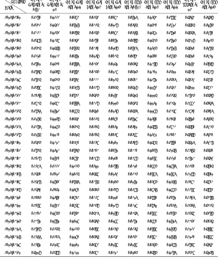
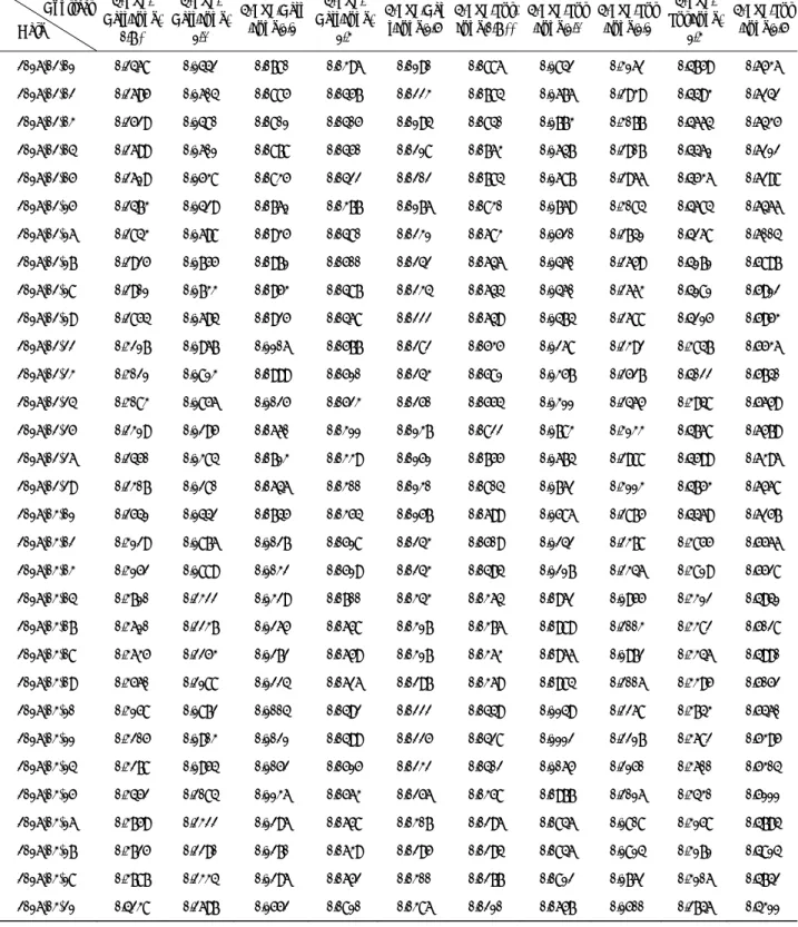
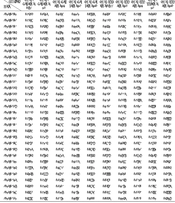
previous 500 trading days. Table C1 (see Appendix C) shows the results of the estimated parameters for the
63‐day period using the MCMC‐LV method.
As shown in Table C1, each trading day has a unique set of parameters. The training samples for the
parameters on each day are the 50ETF closing prices and the O/N SHIBOR rates over the previous 500 trading days.
Therefore, the parameters for the different trading days are similar, but not the same. With regard to the parameters
of the 50ETF closing prices, the drift rate denotes the ability to achieve long‐term stable returns. Because the
training samples are all taken from a b