RNA-Seq Data via Feature Clustering
and Selection
Edwin Vans1,2(B), Alok Sharma1,5,6,7, Ashwini Patil8, Daichi Shigemizu3,4,5,6, and Tatsuhiko Tsunoda4,5,6
1 School of Engineering and Physics, University of the South Pacific, Suva, Fiji
[email protected], [email protected]
2 School of Electrical and Electronics Engineering, Fiji National University, Suva, Fiji
3 Medical Genome Center, National Center for Geriatrics and Gerontology,
Obu, Aichi 474-8511, Japan
4 Department of Medical Science Mathematics, Medical Research Institute,
Tokyo Medical and Dental University (TMDU), Tokyo 113-8510, Japan
5 RIKEN Center for Integrative Medical Sciences,
Yokohama, Kanagawa 230-0045, Japan
6 CREST, JST, Tokyo 113-8510, Japan
7 Institute for Integrated and Intelligent Systems, Griffith University,
Brisbane, QLD 4111, Australia
8 Institute of Medical Science, University of Tokyo, 4-6-1, Shirokanedai, Minato-ku,
Tokyo 108-8639, Japan
Abstract. We present FeatClust, a software tool for clustering small sample size single-cell RNA-Seq datasets. The FeatClust approach is based on feature selection. It divides features into several groups by per-forming agglomerative hierarchical clustering and then iteratively clus-tering the samples and removing features belonging to groups with the least variance across samples. The optimal number of feature groups is selected based on silhouette analysis on the clustered data, i.e., selecting the clustering with the highest average silhouette coefficient. FeatClust also allows one to visually choose the number of clusters if it is not known, by generating silhouette plot for a chosen number of groupings of the dataset. We cluster five small sample single-cell RNA-seq datasets and use the adjusted rand index metric to compare the results with other clustering packages. The results are promising and show the effectiveness of FeatClust on small sample size datasets.
Keywords: Single-cell RNA-Seq
·
Hierarchical clustering·
Feature selection1
Introduction
Single-cell RNA sequencing (RNA-Seq) is at the cutting edge of cell biology. It quantifies the gene expression profile of the whole transcriptome of individ-ual cells. Analysis of single-cell RNA-seq data through unsupervised clustering
c
Springer Nature Switzerland AG 2019
A. C. Nayak and A. Sharma (Eds.): PRICAI 2019, LNAI 11672, pp. 445–456, 2019. https://doi.org/10.1007/978-3-030-29894-4_36
enables researchers to identify cell type and function and to discover heterogene-ity within the cell populations. Heterogeneheterogene-ity within a cell population is common [11] and it occurs in a variety of different cell populations such as tumor cells [10,24], embryonic stem cells (ESCs) [21], hematopoietic stem cells (HSCs) [12] and T cells [5].
Recently, several clustering software packages were developed for analysis of single-cell datasets. One such software package is called SEURAT, developed by Satija Labs for analysis of single cell data-sets [6,18,20]. The original version of SEURAT used PCA on highly variable genes. It then selected statistically significant principal components and projected these to two-dimensional space using t-SNE. Density clustering (DBSCAN) algorithm was then used to identify clusters. The newer version of SEURAT uses PCA and graph-based clustering similar to [16,26].
ˇ
Zurauskien˙e and Yau [28] developed a hierarchical clustering based method which they called pcaReduce. pcaReduce works by first reducing the dimension-ality of the gene expression matrix to k−1 using PCA, where k is the initial cluster size. It then usesk-means to divide the data intok clusters and obtains the mean and the covariance matrix for each cluster. pcaReduce does the follow-ing steps in a loop. A probability distribution based on multivariate Gaussian is used to find the probability of merging pairs of clusters for every possible pair of clusters. The pair with the highest probability is merged. The principal compo-nent in the reduced data that explains the least variance is removed iteratively. The mean and covariance are updated, and the algorithm repeats until only one principal component is left.
A recently developed software package for clustering of single cell data is called SC3 [15]. The SC3 package utilises three different metrics for calculation of the distance between cells. They use Euclidean, Pearson’s and Spearman’s distances. Also, the authors use PCA and graph Laplacian for transforming the data into a lower dimensional space. They then usek-means and select some clusterings corresponding to the reduced dimension for consensus. They choose a range of reduced dimensions and finally perform consensus using various results. While the consensus approach improves clustering accuracy and provides stable cluster assignments, the method is very complicated to use for small datasets.
The clustering packages described here use either centroid based k -means clustering, connectivity based hierarchical clustering or graph-based clus-tering. The k-means clustering algorithm also commonly referred to as Lloyd’s algorithm [17] finds k centroids and assigns each of the samples to its closest centroid to minimise the sum of the squared distance between the centroids and each of its assigned sample point. While thek-means clustering algorithm does converge in findingkoptimal centroids or means, it can get stuck in local min-ima. Another problem is that different initialisation can result in different cluster centroids, which makes the algorithm unstable. Hence, thek-means algorithm is usually run a few times using different initialisation. Thekcluster means are the parameters of the algorithm, and it can be initialised by randomly choosing k
samples from the dataset. There are numerous initialisation methods. However, one favorite initialisation technique is kmeans++ [3].
Connectivity-based methods such as hierarchical clustering work by dividing the data points into a hierarchy of clusters. A standard version is agglomerative hierarchical clustering which is the bottoms up approach. Initially, each data point in the training set is its cluster. In other words, all the clusters initially are singletons. Subsequently, pairs of clusters are merged at each step of the algorithm by minimising the linkage criterion until only one cluster remains (containing all the data points). One useful measure is Ward’s criterion [25]. Ward’s criterion merges two clusters by minimising their within-cluster variance. Thus it is also known as minimum variance criterion. Hierarchical clustering, while giving very stable groupings is prone to noise which can lead to incorrect clusters of the data. Furthermore, computational requirements increase with increasing number of samples.
based clustering methods treat samples as nodes in a graph. Graph-based clustering methods identify groups of nodes that are highly connected, for example, by constructing a k-nearest neighbour graph. Two nodes can be combined if they share at least one nearest neighbour (shared nearest neighbour). The kin k-nearest neighbour graph affects how many clusters are detected. In the results section, we describe how we used SEURAT which uses graph-based clustering to obtain the desired number of groups. Graph-based methods are more suited to large datasets with a high number of samples.
One of the challenges in clustering single-cell RNA-Seq data is the high dimensionality of the genes in the dataset. For clustering purposes, genes which are expressed in all the cells (ubiquitous genes) do not contribute much to deter-mining the groupings of the cells. On the other hand, genes which are only expressed in a few cells also do not assist to identifying the clusters of the cells. Many of the dimensions also contain noise which can prevent correct clustering of the sample cells. Removing these genes is one way of reducing the dimen-sionality of the dataset to some extent. This approach is called gene filtering, and many clustering packages such as SC3 and SEURAT use this approach for reducing data dimensionality.
Popular clustering packages discussed here perform feature extraction through PCA, t-SNE or graph Laplacian-based methods prior to clustering. Through such techniques, the features are projected to a lower dimensional space which contains essential information in the data and the dimensions that include noise are removed. Also, these methods do not require grouping information of the samples to be known a priori. On the other hand, selecting important fea-tures through feature selection for clustering of single cell data has not been explored much. Feature selection involves applying a statistical technique to select informative features or genes in the data. For example, genes with the high-est variance across cells could be instructive in determining cell type. Through feature selection, features which do not give valuable information for clustering the samples, or noisy features may be removed.
In this paper, we explore the idea of feature selection for reducing the high dimensionality of gene expression data and for improving clustering accuracy. We propose the concept of first clustering similar features in the data into groups, finding the mean of the feature groups and then iteratively removing those groups of features from the dataset which contain low cluster mean variance across the samples. FeatClust selects the optimal number of feature groups by performing silhouette analysis; that is, computing silhouette score in each iteration after the clustering the samples. FeatClust can additionally generate silhouette plots that can be used to visually determine the number of clusters if it is not known. The method is simple to understand and easy to implement. Also, the clustering results on five small sample single-cell datasets show that this approach success-fully removes less informative features and improves clustering accuracy. This paper is organized as follows. Section2 describes the method in more details. Section3 presents the clustering results of the technique on three small sample datasets and provides a discussion of the results. Section4draws the conclusions and recommendations for future work.
2
FeatClust Method
The proposed FeatClust method takes an iterative feature elimination approach where we first cluster features into some groups and then iteratively remove less important groups of features. The proposed algorithm is given in Algorithm1. The input to the proposed approach is the gene expression matrix X which is ad×nmatrix wheredrepresents features (or genes), andnrepresents samples (or cells) and the number of clusters q, which is known a priori. The output
ysamples is an-dimensional vector which contains the cluster labels in the range [1,2, ..., q] of each cell inX.
2.1 Gene Filtering and Normalization
As a pre-processing step, we take the counts or the normalised counts matrix where rows represent genes and columns represent cells and apply log transfor-mation after adding a pseudo-count of 1. Thus we get X = log2(counts + 1). A gene filter is applied which rejects highly and lowly expressed genes. The gene filter removes genes expressed (expression value>0) in less thanr% of cells and genes expressed in greater than (100−r)% of the cells. By default we choose
r= 10 as ubiquitous and rare genes do not provide much information to improve clustering. This reduces the dimensionality of the cells, thus increasing the com-putational speed of the method. Finally, the features are normalised to the L2 unit norm. This is done by computing the L2 norm across all samples for each feature and then dividing the feature by the L2 norm.
2.2 Feature Clustering
The proposed approach starts by clustering the features of the input X into
Algorithm 1.Proposed FeatClust Algorithm Input:X a (d×n) gene expression matrix,qandk
Output:ysamples∈ {1,2, ..., q}, ann-dimensional vector of cluster labels of the
samples
1 Cluster the features ofX intokgroups using agglomerative clustering
2 For thek feature groups compute cluster centres to getμi, wherei= 1,2, ..., k andμiis a n-dimensional vector
3 Compute the varianceσ2i ofμiacross samples
4 X ←X
5 i←0
6 forj=ktoqdo
7 Perform hierarchical clustering on samples ofX, yi←hierarchical clustering(X, q)
8 s scorei←silhouette score(X, yi)
9 Remove all features fromX belonging to feature group having lowest cluster mean variance so that onlyj−1 feature clusters remain
10 i←i+ 1
11 index←arg max i s scorei
12 ysamples←yindex
d, then we have singleton clusters of the features. Setting a very large value of kcan slow down the algorithm while on the other hand setting a very small value can result in the algorithm not being able to properly separate and remove low variance features. We suggest setting k to about 20% ofn to create a bal-ance between removing less informative features and computational speed of the algorithm. The features are then clustered using agglomerative hierarchical clustering employing Ward linkage criterion and Euclidean distance measure. Once the features are clustered into groups, the cluster centres of thek groups are computed resulting in μi which is an-dimensional vector. The varianceσ2i,
where i= 1,2, ..., k, across samples of each of the feature cluster means is also computed.
The proposed approach then iteratively clusters the samples, again using hierarchical clustering employing Ward’s criterion, computes the silhouette score using the cluster labels obtained through hierarchical clustering and then removes the feature group which has the least variance of the cluster means. The iteration starts with allkgroups of features and stops whenqgroups of features remain.
2.3 Optimal Feature Groups
The silhouette score is computed as the mean of individual silhouette coefficient of the samples. The silhouette coefficient for each sample is computed as follows
S= sn−sw
where sw is the mean within cluster distance and sn is the mean nearest
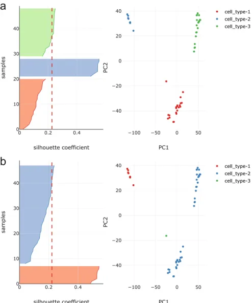
clus-ter distance for the sample. Usually, silhouette analysis is done to declus-termine the number of clusters in the dataset visually. We also use silhouette analysis to determine the optimal number of groups of features. To select the optimal number of feature groups, we take the clustering which gives the maximum sil-houette score. In addition to clustering, the FeatClust method provides functions to visualise the clustering result as silhouette plots, and its corresponding 2D scatter plot. Figure1shows silhouette and its relevant PCA scatter plots in 2D generated by FeatClust for two different clustering results. It is seen that the average silhouette score of all the samples (depicted by the red dashed line) is greater in the plots corresponding to higher ARI score.
3
Results
We tested our clustering method five small sample single cell datasets containing very high dimension. Here we define small sample datasets as datasets having less than 200 samples. These datasets include Biase et al. [4], Yan et al. [27], Goolam et al. [8], Fan et al. [7] and Treutlein et al. [22]. The Biase et al., Goolam et al. and Fan et al. datasets contain single cells from various stages of mouse embryo development. The Yan et al. dataset contains single cells from human preimplantation embryos, and embryonic stem cells and the Treutlein et al. dataset contains single cells from various mouse tissues. A summary of the datasets is given in Table1.
Table 1.Summary of single cell datasets used in experiments. The last column, clus-ters, refers to the number of different cell types in the dataset as reported by the original authors.
Dataset Features (genes) Samples (cells) Clusters
Biase 25737 49 3
Yan 20214 90 7
Goolam 41480 124 5
Fan 26357 66 6
Treutlein 23271 80 5
The datasets were downloaded in RSingleCellExperiment object format from [1]. The counts/normalised counts and column/row meta-data (e.g., names of genes etc.) were extracted from SCE object and stored in comma-separated values (CSV) files to be accessed by our Python script. We compared our method with the various recent state of the art single cell clustering packages such as SEURAT, SC3, SIMLR [23], pcaReduce, SINCERA [9] and TSCAN [13]. We applied the same pre-processing and normalisation steps as we did in our method to the datasets before running the clustering functions of various methods.
Fig. 1. Silhouette plot and the corresponding PCA 2D scatter plot for Biase et al. dataset for two different clustering results; (a) result with ARI of 0.95 and (b) result with ARI of 0.37. The cells are clustered and labelled by our clustering method, Feat-Clust. The red dotted lines show the average silhouette score for all the samples. The average silhouette score is slightly higher for (a) thus FeatClust selects clustering obtained in (a). One can see that (a) is a better clustering result than (b) because more samples in (a) have higher than average silhouette score and the 2D scatter plot differentiates between the three clusters in the dataset. (Color figure online)
The SEURAT R package was installed using the instructions on [2] on 5 December 2018. To run SEURAT’s clustering algorithm on the datasets, we first imported the RDS datasets which were downloaded earlier. The gene expres-sion matrix was extracted, and a SEURAT object was created using the gene expression matrix. PCA was performed separately on the SEURAT object before performing clustering. The SEURAT clustering algorithm had several parame-ters which we set as follows. All default values of the FindClusparame-ters function were used except for the three parameters; k, resolution and the number of prin-cipal components to use in the clustering algorithm. k defines the number of neighbours for thek-nearest neighbour algorithm. Resolution parameter can be used to adjust the number of clusters. The resolution and the number of prin-cipal components to use was set to 1 and 1:10 (this means use first 10 PC’s) respectively. Thekparameter was adjusted experimentally to obtain the desired number of clusterings.
The SC3 R package was downloaded and installed from Bioconductor on 19 September 2018. Since SC3 works on single cell experiment (SCE) objects, a SingleCellExperimentlibrary and class are needed to create SCE objects and pass it to the SC3 function. The originally downloaded datasets were already SCE objects. Thus, we passed these objects to SC3 function to test SC3. The parameters of SC3 for various datasets were set as follows. The first parameter isks where we can either give a range of values or a single value. This parameter sets the number of clusters in the SC3 algorithm. For each dataset, we knew the number of clusters. We set this parameter as a single value representing the number of clusters for each dataset. The second parameter isbiology. We set this as FALSE since we only wanted to test the clustering part of SC3.
The SIMLR R package was downloaded and installed from Bioconductor on 3 March, 2019. An R script was written to test the SIMLR clustering method on the datasets that we have obtained. We followed the examples given in [19] to test SIMLR on our datasets. The parameters of SIMLR were set as follows. The X parameter was set to the preprocessed and normalized gene expression matrix. Thecparameter was set to the actual number of clusters in the dataset. Thek parameter which is the tuning parameter was set to default value of 10. The rest of the parameters were set to defaults.
The pcaReduce clustering package was downloaded from GitHub https:// github.com/JustinaZ/pcaReduce on 4 March 2019 and installed using the instructions in the readme file. An R script was developed to test the pcaRe-duce method. The pcaRepcaRe-duce algorithm had four arguments. The first is theD t which is the dataset argument. We provided the filtered and normalised gene expression matrix. The second parameter is nbt which is the number of times to perform the pcaReduce algorithm. This parameter was set to 100. The next argument isqwhich refers to the number of reduced dimension to start pcaRe-duce. This parameter was set to the default 30. The last parameter of pcaReduce is the method parameter. We set it to the character value ‘S’ which means to perform sample-based merging of clusters.
The SINCERA package was installed on 4 March 2019 following the instruc-tions on their GitHub page https://github.com/xu-lab/SINCERA. An R script was written to test the method on our selected datasets following a demonstra-tion file on their GitHub page. To run SINCERA, an S4 object was created using the filtered and normalized data. Then, PCA was run on the S4 object and finally cluster assignment function was run on the S4 object to obtain the clustering of the datasets. For this method, PCA features were used. The clustering method was hierarchical clustering and the first 10 reduced dimensions were used. The default clustering method in SINCERA was used which is hierarchical clustering with Pearson’s correlation distance and average linkage.
The TSCAN package in R was installed directly from Bioconductor on 3 March, 2019. The TSCAN reference manual [14] was followed and an R script was implemented to test the method on our selected datasets. The TSCAN method was relatively simple to test. There is one function exprmclust which runs TSCAN clustering on the datasets directly. We passed the filtered and nor-malized gene expression matrix, together with the target number of clusterings (clusternum) into this function. The rest of the parameters were defaults.
The results were compared using the adjusted rand index (ARI) metric which compares two different clusterings. The ARI is defined as follows. Given a set of
nsamples in the data and two clusterings of these samples, the overlap between the two groupings can be summarized in a contingency table, where each entry
nij represents the number of samples in common betweeni-th group of the first clustering and thej-th group of the second clustering. The adjusted rand index is computed as follows ARI = ij nij 2 −iai 2 j bj 2 /n2 1 2 i ai 2 +jbj 2 −iai 2 j bj 2 /n2 (2)
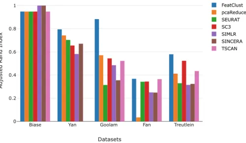
where ai and bj are the sums of rows and columns of the contingency table respectively. The ARI values are in the range [−1,1]. A value of 1 indicates per-fect grouping. A value of 0 indicates a random assignment of samples to groups, and negative values indicate wrong cluster assignments. For all the datasets we computed the ARI between the cluster assignments obtained by the methods and the original groupings of the samples into cell types. We performed 100 trials for each method on all the datasets as some methods included a random component. The results reflect the median of 100 trials. The ARI of our approach and various methods are shown as a bar plot in Fig.2. Compared to the rest of the methods FeatClust performed better in four out of the five datasets.
Fig. 2.Bar plot showing the ARI score for various methods on five datasets. FeatClust performs better in clustering in four out of five datasets compared to the rest of the methods. Note that no results for the method TSCAN on the Yan et al. dataset was obtained.
4
Conclusion
We have presented FeatClust, a software tool for clustering and visualisation of small sample size single-cell RNA-seq datasets containing high dimensionality. The method is based on feature selection by iteratively removing groups of fea-tures which give less information for performing clustering on the samples. The feature clustering and sample clustering is both performed using agglomerative hierarchical clustering employing Ward linkage criterion. The FeatClust method on each iteration removes the feature cluster group giving least variance, where the variance across samples of the cluster means is computed. The result in terms of ARI on five selected datasets shows the effectiveness of the proposed approach. The FeatClust method can also be applied to cluster larger sample datasets. However, the computation speed will reduce if the sample size increases as the method clusters features also. To take advantage of FeatClust’s good clus-tering capability, we recommend using it in a hybrid approach where a smaller subset of cells can be sampled uniformly from large datasets and clustered using FeatClust. The remaining cells can be classified using supervised learning.
Software Availability.The FeatClust algorithm was implemented in Python programming language and is available on GitHub https://github.com/ edwinv87/featclust. The installation and usage instructions are provided on the readme file on GitHub.
References
1. Single-cell RNA-seq datasets. https://hemberg-lab.github.io/scRNA.seq. datasets/. Accessed 08 Sep 2018
2. SEURAT: R toolkit for single cell genomics (2018).https://satijalab.org/seurat/. Accessed 5 Dec 2018
3. Arthur, D., Vassilvitskii, S.: k-means++: the advantages of careful seeding. In: Eighteenth Annual ACM-SIAM Symposium on Discrete Algorithms (2007) 4. Biase, F.H., Cao, X., Zhong, S.: Cell fate inclination within 2-cell and 4-cell mouse
embryos revealed by single-cell RNA sequencing. Genome Res.24(11), 1787–1796 (2014).https://doi.org/10.1101/gr.177725.114
5. Buettner, F., et al.: Computational analysis of cell-to-cell heterogeneity in single-cell RNA-sequencing data reveals hidden subpopulations of single-cells. Nat. Biotechnol. 33(2), 155–160 (2015).https://doi.org/10.1038/nbt.3102
6. Butler, A., Hoffman, P., Smibert, P., Papalexi, E., Satija, R.: Integrating single-cell transcriptomic data across different conditions, technologies, and species. Nat. Biotechnol.36(5), 411–420 (2018).https://doi.org/10.1038/nbt.4096
7. Fan, X., et al.: Single-cell RNA-seq transcriptome analysis of linear and circular RNAs in mouse preimplantation embryos. Genome Biol.16(1) (2015).https://doi. org/10.1186/s13059-015-0706-1
8. Goolam, M., et al.: Heterogeneity in Oct4 and Sox2 targets biases cell fate in 4-cell mouse embryos. Cell165(1), 61–74 (2016).https://doi.org/10.1016/j.cell.2016.01. 047
9. Guo, M., Wang, H., Potter, S.S., Whitsett, J.A., Xu, Y.: SINCERA: a pipeline for single-cell RNA-seq profiling analysis. PLOS Comput. Biol.11(11), e1004575 (2015).https://doi.org/10.1371/journal.pcbi.1004575
10. Hebenstreit, D.: Methods, challenges and potentials of single cell RNA-seq. Biology 1(3), 658–667 (2012).https://doi.org/10.3390/biology1030658
11. Islam, S., et al.: Characterization of the single-cell transcriptional landscape by highly multiplex RNA-seq. Genome Res. 21(7), 1160–1167 (2011). https://doi. org/10.1101/gr.110882.110
12. Jaitin, D.A., et al.: Massively parallel single-cell RNA-seq for marker-free decom-position of tissues into cell types. Science343(6172), 776–779 (2014).https://doi. org/10.1126/science.1247651
13. Ji, Z., Ji, H.: TSCAN: pseudo-time reconstruction and evaluation in single-cell RNA-seq analysis. Nucleic Acids Res.44(13), e117–e117 (2016). https://doi.org/ 10.1093/nar/gkw430
14. Ji, Z., Ji, H.: TSCAN: Tools for Single-Cell ANalysis, October 2018. https:// bioconductor.org/packages/release/bioc/html/TSCAN.html
15. Kiselev, V.Y., et al.: SC3: consensus clustering of single-cell RNA-seq data. Nat. Methods14(5), 483–486 (2017).https://doi.org/10.1038/nmeth.4236
16. Levine, J.H., et al.: Data-driven phenotypic dissection of AML reveals progenitor-like cells that correlate with prognosis. Cell162(1), 184–197 (2015).https://doi. org/10.1016/j.cell.2015.05.047
17. Lloyd, S.: Least squares quantization in PCM. IEEE Trans. Inf. Theory 28(2), 129–137 (1982).https://doi.org/10.1109/tit.1982.1056489
18. Macosko, E.Z., et al.: Highly parallel genome-wide expression profiling of individual cells using nanoliter droplets. Cell161(5), 1202–1214 (2015). https://doi.org/10. 1016/j.cell.2015.05.002
19. Ramazzotti, D., Wang, B., Sano, L.D., Batzoglou, S.: Single-cell Interpretation via Multi-kernel LeaRning (SIMLR), January 2019
20. Satija, R., Farrell, J.A., Gennert, D., Schier, A.F., Regev, A.: Spatial reconstruction of single-cell gene expression data. Nat. Biotechnol.33(5), 495–502 (2015).https:// doi.org/10.1038/nbt.3192
21. Tang, F., et al.: mRNA-seq whole-transcriptome analysis of a single cell. Nat. Methods6(5), 377–382 (2009).https://doi.org/10.1038/nmeth.1315
22. Treutlein, B., et al.: Reconstructing lineage hierarchies of the distal lung epithelium using single-cell RNA-seq. Nature509(7500), 371–375 (2014).https://doi.org/10. 1038/nature13173
23. Wang, B., Zhu, J., Pierson, E., Ramazzotti, D., Batzoglou, S.: Visualization and analysis of single-cell RNA-seq data by kernel-based similarity learning. Nat. Meth-ods14(4), 414–416 (2017).https://doi.org/10.1038/nmeth.4207
24. Wang, D., Bodovitz, S.: Single cell analysis: the new frontier in ‘omics’. Trends Biotechnol.28(6), 281–290 (2010).https://doi.org/10.1016/j.tibtech.2010.03.002
25. Ward, J.H.: Hierarchical grouping to optimize an objective function. J. Am. Stat. Assoc.58(301), 236–244 (1963).https://doi.org/10.1080/01621459.1963.10500845
26. Xu, C., Su, Z.: Identification of cell types from single-cell transcriptomes using a novel clustering method. Bioinformatics31(12), 1974–1980 (2015).https://doi. org/10.1093/bioinformatics/btv088
27. Yan, L., et al.: Single-cell RNA-seq profiling of human preimplantation embryos and embryonic stem cells. Nat. Struct. Mol. Biol.20(9), 1131–1139 (2013).https:// doi.org/10.1038/nsmb.2660
28. ˇZurauskien˙e, J., Yau, C.: pcaReduce: hierarchical clustering of single cell transcrip-tional profiles. BMC Bioinform.17(1) (2016). https://doi.org/10.1186/s12859-016-0984-y