Semi-blind Turbo Detection for Multiple-input Multiple-output Wireless Systems

GOEL,VIVEK. Semi-blind turbo detection for Multiple-input Multiple-output wire-less systems. (Under the direction of Dr. Huaiyu Dai)

Multiple-input multiple-output (MIMO) techniques constitute the core of future high speed wireless systems. Blind detection in MIMO wireless systems conserves bandwidth and is better suited for use in multiple user scenarios. Since, most of the modern wireless communication systems employ some form of forward error correc-tion, therefore, we can exploit the turbo principle to further improve the performance of blind detection schemes for MIMO.

In this thesis we propose a new semi-blind turbo multiuser detector (MUD) for signal detection in a MIMO wireless system, operating on a single link with Gaussian noise. This turbo MUD (named as T-MUK) performs a sub-optimal joint detection and decoding by iteratively exchanging soft information between the detector stage, that optimizes multiuser kurtosis maximization criterion, and the decoder stage, that runs maximum aposteriori probability (MAP) algorithm. It is shown to achieve good performance at the expense of very few training symbols.

by

Vivek Goel

A thesis submitted to the Graduate Faculty of North Carolina State University

in partial satisfaction of the requirements for the Degree of Master of Science in Electrical Engineering

Department of Electrical And Computer Engineering

Raleigh

2005

Approved By:

Dr. Huaiyu Dai

Chair of Advisory Committee

Dedication

Biography

Acknowledgements

Contents

List of Figures vii

List of Symbols ix

1 Introduction 1

1.1 Motivation . . . 1

1.2 Multiple-Input Multiple-Output Systems . . . 2

1.3 Blind Detection . . . 5

1.3.1 Why blind? . . . 5

1.3.2 Blind deconvolution/Blind equalization . . . 6

1.3.3 Classification of blind equalization techniques . . . 8

1.3.4 Blind source separation (BSS) . . . 10

1.3.5 Classification of BSS techniques . . . 11

1.3.6 Similarities and differences between BSS and BE . . . 13

1.3.7 Blind MIMO detection . . . 13

1.4 Turbo Detection . . . 15

1.4.1 Turbo principle . . . 15

1.4.2 Turbo multiuser detection . . . 16

1.5 Thesis Overview and Organization . . . 19

2 Turbo Multiuser Kurtosis Maximization 21 2.1 Multiuser Kurtosis Maximization (MUK) Criterion . . . 22

2.1.1 MIMO system model . . . 22

2.1.2 Necessary and sufficient conditions for BSS . . . 23

2.1.3 MUK criterion and MUK algorithm . . . 26

2.1.4 Channel whitening . . . 28

2.2 Turbo-MUK for Single-User MIMO . . . 29

2.2.1 Detector stage . . . 31

2.2.2 Decoder stage . . . 34

2.3 Turbo-MUK for Multi-User MIMO . . . 37

2.5 Summary . . . 43

3 Semi-Blind interference cancellation 44 3.1 Introduction . . . 44

3.2 Multicell MIMO System Model . . . 45

3.3 Group Successive Interference Cancellation . . . 47

3.4 T-BLAST . . . 49

3.5 Semi-Blind Successive Interference Cancellation . . . 50

3.6 Numerical Results . . . 52

3.7 Summary . . . 62

4 Conclusions and Future work 63 4.1 Conclusions . . . 63

4.2 Future Work . . . 64

List of Figures

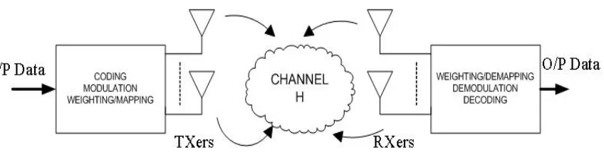
1.1 Diagram of MIMO wireless system. Coding, modulation, and mapping

of the signals onto antennas may be realized jointly or separately. . . 2

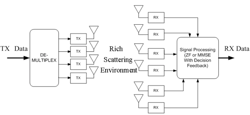
1.2 V-BLAST System Model . . . 4

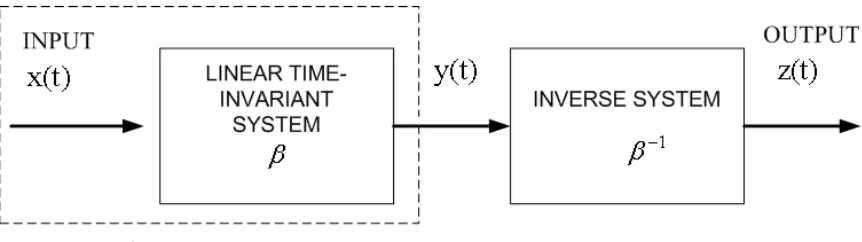
1.3 Block Diagram for Blind Deconvolution . . . 7

1.4 Block Diagram for Blind Source Separation . . . 10

1.5 Transmitter Configuration for Turbo-MUD . . . 17

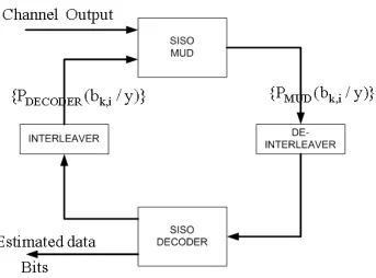
1.6 General Receiver Structure for Turbo-MUD . . . 18

2.1 Instantaneous Linear Mixture Setup . . . 24

2.2 Structure of Turbo-MUK for single-user MIMO system . . . 30

2.3 Structure of Turbo-MUK for multi-user MIMO system . . . 37

2.4 Performance of Single-User Turbo-MUK . . . 41

2.5 Performance of Multi-User Turbo-MUK (Unequal Powers) . . . 42

3.1 Multicell MIMO system (downlink). Each transmitter hasN_tantennas and each receiver has N_r antennas . . . 45

3.2 Multicell MIMO system model. Each interfering transmitter has a single antenna and each receiver has N_r antennas . . . 47

3.3 Effect of asynchronous training sequences . . . 49

3.4 Structure of T-BLAST . . . 50

3.5 Semi-blind group interference cancellation detector . . . 51

3.6 Results for a multicell system having interferers with multiple anten-nas, where the strongest interferer is 6db stronger than other interferers. 53 3.7 Results for a multicell system having interferers with multiple anten-nas, where the strongest interferer is 9db stronger than other interferers. 54 3.8 Results for a multicell system having 4 adjacent cell interferers with single antenna, where the strongest interferer is 3db stronger than the weakest interferer. . . 56

3.10 Results for an interference-limited multicell system having interferers with multiple antennas, where the strongest interferer is 6db stronger than other interferers. SIR = 1db . . . 58 3.11 Results for an interference-limited multicell system having interferers

with multiple antennas, where the strongest interferer is 9db stronger than other interferers. SIR = 0db . . . 59 3.12 Results for an interference-limited multicell system having 4 adjacent

cell interferers with single antenna, where the strongest interferer is 3db stronger than the weakest interferer. SIR =2db . . . 60 3.13 Results for an interference-limited multicell system having 6 adjacent

List of Symbols

Symbol

Definition

{.}T _{Transposition}

{.}∗ Conjugation

{.}H _{Hermitian transpose (i.e., Conjugate transpose)}

{.}† Moore-Penrose Pseudoinverse

{.}−1 Inverse

E{.} Expectation operator

|.| Absolute value (Modulus) Bold Face Letter Matrix

Capital Letter Column or Row vector

σ_{.} Variance

K{.} Kurtosis

sign Signum function

∇ Gradient operator

Chapter 1

Introduction

1.1

Motivation

computa-Figure 1.1: Diagram of MIMO wireless system. Coding, modulation, and mapping of the signals onto antennas may be realized jointly or separately.

tional cost. Alternatively, turbo principle can be explored to achieve near-optimal performance at a much lower computational complexity, and is incorporated in our study. In the next few sections we will give an overview of MIMO communication, blind detection and the turbo principle.

1.2

Multiple-Input Multiple-Output Systems

multiple independent information streams in parallel (known as the spatial multiplex-ing gain) over a matrix channel created by multiple transmit and receive antennas. Whereas, the increase in quality (or BER minimization) is due to the ability of a MIMO system to utilize the spatial dimension to combat adverse channel conditions (known as the diversity gain).

In order to explain the spatial multiplexing gain in MIMO, consider a wireless system with N_t transmit antennas and N_r receive antennas. At the transmitter N_t data streams are transmitted that mix together in the wireless channel as they use the same frequency spectrum. At the receiver, the objective is to estimate the mixing channel matrix (through training symbols) and to separate individual data streams. Assuming flat-fading channels, that is, each entry of the channel matrix is a scalar coefficient, the separation of data streams is possible only if each receive antenna sees a sufficiently different channel. A highly scattering environment resulting in rich multipath ensures that this condition is satisfied. The key point here is that unlike conventional single-input single-output (SISO) wireless systems where multipath rep-resents an impediment to accurate transmission, MIMO actually exploits multipath to maximize the data rate over a given transmission link. Spatial multiplexing in MIMO is somewhat similar to code-division multiple access (CDMA) transmission in which multiple users/streams share the same time/frequency channel upon transmis-sion and are recovered through their unique codes (signatures). The main difference is that in MIMO, unique spatial signatures of input streams exist naturally due to rich multipath, thus using available spectrum more efficiently.

Figure 1.2: V-BLAST System Model

an actual MIMO system depends on the the system architecture and communication environment.

The capacity of a MIMO system with N_t transmit and N_r receive antennas with no transmit channel state information (Foschini & Gans mar. 1998), (Telatar june 1995) is given by

C =log₂[det(I_Nr + ρ N_tHH

H_{)] b/s/Hz, (1.1)}

where H denotes the transpose-conjugate, H is the channel matrix, ρ is the SNR at any receive antenna and we assume N_t uncorrelated equal-power sources. Fos-chini and Telatar both demonstrated that the capacity in (1.1) grows linearly with n=min(N_t, N_r) under certain channel conditions. This information theoretic result serves as an upper bound for actual algortihms/architectures for MIMO developed to achieve a given BER and data rate at a reasonable complexity.

(Foschini 1996) utilizes a diagonally layered coding structure at the transmitter in which code blocks are dispersed across diagonals in space-time. In an independent Rayleigh environment, this processing structure can achieve rates approaching 90% of the Shannon capacity. Vertical-BLAST (Wolniansky, Foschini, Golden & Valen-zuela oct. 1998) is the most likely architecture (Figure 1.2) to be utilized in future wireless systems due to its low complexity and ease of implementation. In V-BLAST (without forward error correction), the encoding process for transmitted data is sim-ply a demultiplex operation followed by independent bit-to-symbol mapping of each substream. Whereas, at the receiver conventional adaptive antenna array techniques (e.g. minimum mean square error (MMSE), zero forcing (ZF)) are used, to detect one substream at a time and null remaining substreams, in conjugation with succes-sive cancellation (cancelling out detected components of the transmit vector from the received signal vector) in a manner analogous to the decision feedback equalization. A recent addition to this class of architectures is turbo-BLAST (Section 1.4), which can achieve rates very close to shannon capacity by better exploitation of transmit and receive diversity.

1.3

Blind Detection

1.3.1

Why blind?

Blind techniques have been actively studied over the past 25 years. Many algo-rithms have been proposed in the context of blind equalization and signal separation. The goal of blind estimation is to determine the channel or the signals based on the prior temporal or spatial knowledge. Although, the use of training sequences is probably the most robust way to estimate the channel, there are several reasons for studying blind algorithms:

• Bandwidth is conserved by eliminating or reducing training set.

• Severe multipath fading during the training period can lead to poor channel estimates.

• Training for interference is often not accessible.

• Training requires synchronization, which may not be feasible in multi-user sce-narios.

• In communication intelligence, training is not available.

• In distributed networks, it may not be feasible to send training sequences each time when a new communication link is set up.

Blind algorithms also suffer from some drawbacks as compared to non-blind tech-niques. In general, blind algorithms tend to be computationally more expensive. Due to the non-linear nature of the blind estimation, many proposed methods converge to a local rather than a global minimum. Also, uniqueness of signal estimates may not be guaranteed if small data lengths are used. All blind algorithms result in an inher-ent phase and ordering ambiguity in recovered signals. Apart from the first one, all other problems can be resolved by using a short list of training signals. Although the algorithms are no longer blind, they retain many of the advantages associated with blind algorithms. Hence, purely blind and non-blind methods correspond to the two extremes of an array of possible algorithms. In practice, ideas from both approaches can be combined to minimize the training signal requirement of non-blind methods, and yet obtain the robustness of blind methods at low computational costs.

1.3.2

Blind deconvolution/Blind equalization

Figure 1.3: Block Diagram for Blind Deconvolution

ordinary deconvolution. Consider an unknown linear time-invariant (LTI) system β with input x(t) assumed to consist of independent and identically distributed (i.i.d.) symbols. The only thing known about the input is its probability distribution. The requirement is to restore x(t), or equivalently to identify the inverseβ−1 of the system β, as depicted in Figure 1.3.

require deconvolution are non minimum-phase. In such cases blind deconvolution (BD) is a non-trivial signal-processing task and thus requires use of more complex algorithms. In communication literature deconvolution of the channel output is more commonly known as equalization, therefore in all further discussions the term blind equalization (BE) is used in place of blind deconvolution (BD).

1.3.3

Classification of blind equalization techniques

Blind channel equalization has received considerable attention in communication and signal-processing literature. Higher order statistics (HOS) based BE, second order statistics (SOS) based BE and subspace based BE are some of the widely used (among numerous other) approaches listed in literature for blind identification of the inter-symbol interference (ISI) channel and/or the transmitted signal.

1990) is based on multiuser kurtosis maximization criterion. Here the blind equalizer is computed by stochastic gradient maximization of the kurtosis of the equalizer out-put (K(z_n) =E(|z_n|4)−2E2(|z_n|2)− |E(z2_n)|2) under the constraint that product of the channel vector (H) and the equalizer vector (W), G = HTW is unitary. Apart from these there are a number of other HOS based blind equalization methods (Sato june 1975), (Hatzinakos & Nikias jan. 1989), (Tugnait may 1987) etc.

In (Gardner june 1991), it is shown that SOS of cyclostationary signals contain phase information which can be used for the identification of non-minimum phase systems. This led to the development of algorithms which explore the cyclostationary properties of oversampled communication signals to allow the blind estimation to be accomplished based on the SOS of the channel output. The use of SOS translates into lesser number of observations (faster convergence) as compared to HOS based algorithms. The first SOS based algorithm developed (Tong, Xu & Kailath nov. 1991) employs temporal oversampling on the channel output (y_n), while assuming an i.i.d. system input (x_n). It then enforces a Jordan structure on the input correlation matrix (R_xn(k) = E(x_nxH

n−k)) and essentially reconstructs the channel vectors in channel

matrix (H) based on the information provided by the change of rank of R_yn(k) = E(y_nyH

n−k). There are a number of other SOS based blind equalization approaches

listed in the literature (Tong, Xu, Hassibi & Kailath jan. 1995), (Giannakis nov. 1994). The blind identification using SOS has a unique solution provided certain conditions (Tong et al. nov. 1991), (Xu, Liu, Tong & Kailath april 1994) on channel and input are met. Although these SOS based methods perform well in general, they suffer a performance degradation caused by a model mismatch when a limited number of observations are available.

Figure 1.4: Block Diagram for Blind Source Separation

(Slock nov. 1994) depicts the key role of channel structure in blind estimation, it is built on the fact that the column span of the block Toeplitz channel matrix and its corresponding complement are the channel signal subspace and channel signal or-thogonal subspace respectively, which can be caclulated from the channel data matrix. Some other algorithms that exploit channel and signal subspace structures are the least square algorithm (Liu, Xu & Tong nov. 1993) and the signal subspace algorithm (Liu & Xu nov. 1995). The performance of this genre of algorithms is fundamentally limited by the nature of the channel. For example, singularity in the channel matrix can result in the divergence of subspace, and result in failure of subspace approaches.

1.3.4

Blind source separation (BSS)

In order to describe the basic blind signal separation problem, consider a set of unknown source signals x₁(t), x₂(t), . . . , x_m(t) that are mutually independent of each other. These signals are linearly mixed in an unknown environment to produce a m×1 observation vector (see Figure 1.4)

Y(t) = AX(t), (1.2)

vec-tor Y(t), the requirement is to recover the original source signalsx₁(t), x₂(t), . . . x_m(t) without any knowledge about the mixing matrix A. The solution to this problem is feasible, except for an arbitrary scaling of each source signal and possible permutation of indices under certain but fairly general conditions. Given that the original source signals are independent and the mixing matrixAis non-singular, it is possible to find a demixing matrix W defined as follows:

Z =WY =WAX =DPX, (1.3)

where Z is the output signal vector produced by the demixer, D is the non-singular diagonal matrix, andPis the permutation matrix. The underlying principle involved in the solution of this problem is called independent component analysis (ICA), which may be viewed as an extension of widely known principal component analysis (PCA). Whereas PCA imposes independence in a statistical sense only to second order while constraining the direction of the vectors to be orthogonal, ICA imposes statistical independence on all the individual components of the output vector, but has no orthogonality constraint. In general it is possible to blindly recover source signals for an×mmixing matrix, where the n≥mcase can be handled using ICA, however the n < m case requires additional information about sources along with independence of sources.

1.3.5

Classification of BSS techniques

A number of blind source separation algorithms have been proposed in recent past. In this section, we classify some of these algorithms and highlight their common properties. As a first step, BSS algorithms can be broadly classified into two classes based on properties used for channel or signal estimation, which include temporal signal properties such as higher order statistics, finite alphabet, cyclostationarity, and spatial receiver properties such as calibrated array or special array geometry.

an output entropy minimization point of view, and was later expanded in (Comon july 1996) using notion of contrast (a contrast is a cumulant based function of the outputs that is maximized if and only if separation is achieved). Some other methods that rely directly on HOS cumulants were introduced in (Cardoso 1989), (Shamsunder & Giannakis 1994). The HOS based BSS criterion described in (Papadias dec. 2000b) (detailed description given in later chapters) builds upon the kurtosis maximization technique for BE and deflation approach (sources are extracted one by one)(Delfosse & Loubaton apr. 1994a), to give a BSS algorithm that is globally convergent. An-other class of algorithms that use HOS implicitly are constant modulus (CM) type BSS techniques that build upon the CM techniques for BE, notable among these (Vanderveen & Paulraj 1996). Finite alphabet property based BSS algorithms, e.g., (Talwar, Viberg & Paulraj feb. 1994), also use HOS in an implicit sense, which exploit the finite alphabet property of the digital signals to develop a maximum like-lihood approach for estimating transmitted signals from the received instantaneous mixture. Some other algorithms rely on assumption that different sources have dif-ferent cyclostationary features (Agee, Schell & Gardner apr. 1990) or exploit spectral redundancy at the cyclic frequency for source separation (Schell & Gardner 1993).

1.3.6

Similarities and differences between BSS and BE

Blind equalization and blind source separation are the two most important blind signal-processing problems. These problems are somewhat related (evident from the use of similar concepts for developing algorithms for solving them) with similarities and subtle differences between them. In BSS, sources are corrupted by the superpo-sition of other sources, in BE, a source is corrupted by time-delayed versions of itself. In both cases unsupervised (blind) learning must be used because no error signals are available. The most important dissimilarities regarding the nature of BSS and BE are

• The dimension of the source-separation task is equal to or less than the length of the vector Y(k) that is composed of linear mixture of the unknown source signal vector X(k), whereas the dimension of the deconvolution task depends on the length of the impulse response of the unknown LTI system β.

• Source separation can involve m (where m is the number of unknown sources) different source probability distribution functions (pdfs), whereas deconvolution only involves one source pdf. The difference between pdfs in source separation means that solutions to the problem may require estimation of different source pdfs, or detection of difference between source pdfs.

1.3.7

Blind MIMO detection

use some combination of BE and BSS algorithms for extracting source signals out of a convolutive mixture at the receive antenna array. In this thesis, the emphasis is on blind MIMO detection for memoryless channel, but for completeness, we will briefly describe some of the promising detection techniques proposed in recent works for solving the convolutive mixture blind identification problem (FIR-MIMO blind identification).

linear dispersive mixing channel.

In summary, we have seen that there is a wide range of possible techniques for blind MIMO detection, which can be well suited for specific wireless communication applications. The choice of particular technique depends on signal, channel and re-ceiver characterstics. Convergence, computational complexity and ability to track variations in a wireless channel are other important issues taken into account when making this choice.

1.4

Turbo Detection

1.4.1

Turbo principle

about a set of symbols exchanged by decoders is in terms of log of ratios of the prob-ability of a symbol having a particular logical value (Pr{d=1}) to the probability of that symbol not having this logical value (1-Pr{d=1}). This soft information is termed as log likelihood ratio (LLR).

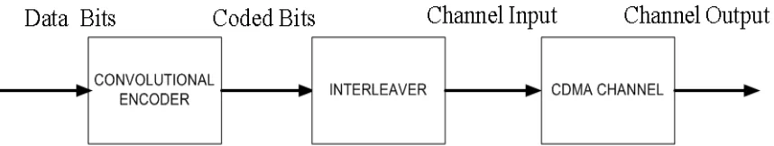
In recent years it has been shown that the turbo principle discussed here in the context of error control coding can be successfully applied to several other complex signal processing problems in digital communications. Notable among these are joint channel equalization and decoding (C. Douillard oct. 1995), joint multiuser detection and decoding (Poor sept. 2001), joint channel estimation and decoding (Komninikas & Wesel sept.2001). The common feature of all these is the use of the turbo structure which involves iterative exchange of soft information about symbols between the two blocks separated by interleavers.

1.4.2

Turbo multiuser detection

The type of communication in which several transmitters share a common channel is known as multiaccess communication. Mobile telephones transmitting to a base station, ground stations communicating with a satellite, and local area networks are a few examples of this type of communication system. A common feature of these com-munication channels is that the receiver obtains a noisy version of the superposition of the signals sent by the active transmitters. A simple solution to avoid this super-position of signals is to ensure an orthogonal multiplexing of signals (various users operate in separate non-interfering channels). But this solution is practically infeasi-ble due to economic considerations and the fact that unintentional superposition of signals is still possible. Thus, in all practical multiacess communication systems users are multiplexed in a non-orthogonal fashion.

wire-Figure 1.5: Transmitter Configuration for Turbo-MUD

line channels such as digital subscriber lines (DSLs) in which crosstalk is the major impairment. The basic idea of multiuser detection is to exploit the cross-correlations among the signals to be demodulated in order to improve the data detection.

Figure 1.6: General Receiver Structure for Turbo-MUD

multiuser detection and decoding is shown to have very good performance. In (Wang & Poor july 1999) such turbo multiuser detectors with maximum likelihood detection (ML) stage and minimum mean square error with parallel interference cancellation (MMSE-PIC) stage have been proposed and shown to have performance close to the single user bound. Here we have discussed the turbo multiuser detection principle in the context of CDMA cellular systems but the same principle is applicable to other cellular systems and applications as well.

These structures have been shown to reach very close to the capacity limit in the interference-free (single cell) case. The detection structures, such as coded V-BLAST and T-BLAST in (Dai et al. mar. 2004), are composed of a BLAST-like MUD stage with soft metric output and a maximum aposteriori probability (MAP) decoding stage, exchanging soft information iteratively (refer to Chapter 3 for more details about T-BLAST). The detection structure in (Sellathurai & Haykin oct. 2002) is more like D-BLAST with a sub-optimal turbo receiver that performs iterative decoding of the random layered space time codes (applied at the transmitter) and estimation of channel matrix in an iterative and simple fashion.

Following the same line of reasoning the turbo principle is applicable for joint MUD and decoding in coded blind MIMO systems, too. The only implementation of such structure we came across in literature is Sequential Monte Carlo (SMC) based turbo receiver for MIMO systems proposed in (Guo & Wang april 2003). This receiver structure uses SMC methodology for blind detection and a MAP decoder in an itera-tive manner in order to approach close to the capacity limit. The SMC methodology recently emerged in the fields of engineering and statistics and can be used in solv-ing a wide class of sophisticated statistical inference problems. Under a state-space framework the SMC recursively generate Monte Carlo samples of the state variable or some other latent variables, based on which the posterior distribution of any param-eter of interest can be approximated. The SMC methods exhibit global convergence and are robust to choice of initial conditions.

1.5

Thesis Overview and Organization

transmitted substreams in single-cell MIMO systems and the interfering substreams (from users in the adjacent cells) in multi-cell MIMO systems in a semi-blind fashion (using minimal number of training symbols), so as to reduce the system overhead and to make these detection structures a better choice for use in broader wireless applications. In multi-cell MIMO systems, the estimation and removal of interfering substreams assists in achieving the main objective, that is to get an improved estimate for symbol substreams transmitted by the desired user.

The thesis is organized as follows. In this first chapter, we have motivated our work in the context of multiple-input multiple-output systems, existing BE/BSS/blind MIMO detection techniques and the concept of turbo MUD. In chapter 2, we will discuss the multiuser kurtosis maximization criterion, a promising idea recently pro-posed for blind MIMO detection, and the stochastic gradient algorithm that can be used to implement this criterion. After this we develop a new semi-blind turbo space-time MUD structure for single-cell MIMO, which we name as turbo - multiuser kurtosis maximization (T-MUK). The detection stage of this turbo MUD structure is a modification of MUK detector such that it can process soft information from the decoder stage with interference cancellation and output soft information to be fed to the decoder. We show that T-MUK structure works even if symbol streams transmitted from different antennas have different power levels. We demonstrate the performance of T-MUK with some numerical results.

Chapter 2

Turbo Multiuser Kurtosis

Maximization

2.1

Multiuser Kurtosis Maximization (MUK)

Cri-terion

2.1.1

MIMO system model

We first consider a single cell MIMO system (no inter-cell interference) and adopt the well known MIMO system model given by

Y(k) =HX(k) +N(k), (2.1)

whereY(k) represents the N_r×1 received signal vector,X(k) = [x₁(k). . . x_Nt(k)]T _is

theN_t×1 transmitted signal vector, Hrepresents theN_r×N_tmatrix which captures channel characteristics between the transmit and the receive antenna arrays,N(k) is the additive background noise vector, all at a time instantk. The transmitted signal power is constrained by E[X(k)H_{X(k)] ≤ P, and the additive background noise is}

circularly symmetric Gaussian with the covariance matrix given by Φ_N =σ2I. The entries of the complex matrix H are independent with uniformly distributed phase and normalized Rayleigh distributed magnitude, modelling a Rayleigh fading channel with sufficient separation between the transmit and the receive antennas. The signal to noise ratio (SNR) is given by ρ=P/σ2.

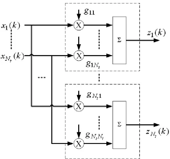
For studying blind methods in MIMO systems, we further assume thatN_tstreams transmitted from N_t antennas are i.i.d., mutually independent, zero-mean discrete time sequences. The objective of the MUK criterion to be discussed in subsequent sections is to recover these symbol streams from the output of the linear channel (H) that introduces inter-stream interference. In order to achieve this objective, the received signal vectorY(k) is filtered by anN_r×N_tmatrix equalizerWthat produces output vector Z(k) = [z₁(k). . . z_Nr(k)]T_,

Z(k) = WTY(k)

= WTHX(k) +N_w(k)

= GTX(k) +N_w(k), (2.2)

and the equalizer matrix), and N_w(k) is the colored noise at the receiver output. In case of perfect signal recovery (in absence of noise) the equalizer ouput vector Z(k) should be an exact replica of the transmitted signal vector X(k), whose components are given by

z_j(k) =

Nt X

l=1

g_jlx_l(k) = GT_jX(k), j = 1, ...., N_t, (2.3)

where G_j (the jth _{column of G) is composed of weighting factors for all the channel}

inputs to the jth equalizer ouput. We can express the same relationship in a more compact vector notation

Z(k) = GTX(k), (2.4)

where

G= [G₁. . . G_Nt]

     

g₁₁ . . . g_Nt1 ..

. ... ... g_1Nt . . . g_NtNt

    

. (2.5)

The above described instantaneous linear mixture setup is shown in Figure 2.1. We define the variance and the kurtosis of equalizer output (needed later to develop the MUK criterion) as follows

E(|z_j|2) =σ_x2

Nt X

l=1

|g_jl|2, j = 1, . . . , N_t (2.6)

K(z_j) =K_x

Nt X

l=1

|g_jl|4, j = 1, . . . , N_t (2.7)

whereK_x =E(|x|4)−2E2(|x|2)− |E(x2)|2 is the unnormalized kurtosis andσ_x2 is the variance of any input substream {x_l(k)} .

2.1.2

Necessary and sufficient conditions for BSS

identically distributed (Cardoso oct. 1998). Thus, we say blind recovery is achieved if, after suitable reordering of the equalizer outputs the following holds

z_j(k) =eiφj_x

j(k), (2.8)

for some φ_j ∈[0,2π) and all j ∈1, . . . , N_t.

If the conditions on the transmitted signals described in the previous section hold, the following set of conditions are necessary and sufficient for the blind recovery of all the transmitted signals at the equalizer outputs:

A1) |K(z_j(k)|=|K_x|, j = 1, . . . , N_t A2) E|z_j(k)|2 =σ_x2, j = 1, . . . , N_t A3) E(z_l(k)z_k∗(k)) = 0, l 6=j.

Proving that the given set of conditions is necessary is quite straightforward, A1 and A2 are evident from (2.8) and A3 follows from the fact that E(x_l(k)x∗_j(k)) = 0 for l6=j. In order to prove that these conditions are sufficient consider the following inequality

l=XNt

l=1

|g_jl|4 ≤(

lX=Nt

l=1

|g_jl|2)2, j = 1, ...., N_t, (2.9)

where the equality holds if and only if there exists a unique non-zero element g_jl of unit magnitude for each j. Now from (2.7), A1 and (2.6), A2 we obtain

l=_XNt

l=1

|g_jl|4 = 1,

l=_XNt

l=1

|g_jl|2 = 1. (2.10)

If we put together the inequality in (2.9) and (2.10), we can see that G_j must be of the form

G_j = [0. . .0eiφj_{0. . .0]}T_{, (2.11)}

where the single non-zero element can be in any arbitrary position. Now combining A3 and (2.4) gives

According to (2.11) and (2.12), theN_tdifferent vectorsG_j of the form shown in (2.11) will contain their unique non-zero elements at different positions, which corresponds to the recovery of all N_t different inputs. Therefore, after reordering we obtain (2.8).

2.1.3

MUK criterion and MUK algorithm

The necessary and sufficient conditions for BSS discussed in the previous section form a basis for the following optimization criterion (known as the multiuser kurtosis maximization criterion) for blind signal recovery

max

| {z }

G

F(G) =

Nt X

j=1

|K(z_j)|

subject to : GHG = I_Nt. (2.13)

The constraint comes from the fact that, conditions A2 and A3 give

E(ZZH) =σ_x2I_Nt. (2.14)

adaptive stochastic-gradient with orthogonalization algorithm discussed here (Papa-dias dec. 2000b) (called the MUK algorithm thus far) is direct on the equalizer parameters, aims at joint recovery of all the sources (for any number of sources) and ensures convergence to the global optimum (even in the presence of Gaussian noise). This convergence to the global optimum is derived assuming channel matrix H to be full-rank, thus the maximum number of streams that can be recovered is limited by the degrees of freedom of the system. In the following we briefly introduce this algorithm. First we rewrite F(G) as

F(G) =

Nt X

j=1

sign(K(z_j))K(z_j)

= sign(K_x)

Nt X

j=1

(E|z_j|4−2E2|z_j|2− |E(z_j2)|2). (2.15)

Assuming symmetrical inputs (E(x2(k) = 0) so thatE(z_j2(k) = 0)

F(G) = sign(K_x)

Nt X

j=1

(E|z_j|4−2E2|z_j|2). (2.16)

By invoking condition A2, E|z_j(k)|2 is a constant, thus the gradient of F(G) with respect to W is given by

∇(F(G)) = 4sign(K_x)

Nt X

j=1

[0_Nr×1, . . . , E(|z_j(k)|2z_j(k)Y∗(k)), . . . ,0_Nr×1], (2.17)

where jth _{term on the right side is a N}

r×Nt matrix with all columns other than jth

column being zero vectors. Now, sum together all the terms on the right side into a single N_r ×N_t matrix and update W in the direction of instantaneous gradient as follows (dropping the expectation operator in (2.17))

W_p(k+ 1) =W(k) +µ sign(K_x)Y∗(k)Z_p(k), (2.18)

whereZ_p(k)) = [|z₁(k)|2z₁(k), . . . ,|z_Nt(k)|2z_Nt(k)]. For the next iteration the orthog-onality constraint for the MUK criterion needs to be satisfied

For this to be feasible we first need to make the channel matrix H unitary. This can be done by using any second order blind separation method (one such method is discussed in the next section) that typically converge to a unitary instantaneous mixture of inputs. Now, in order to satisfy the constraint given by (2.19), it suffices to ensure that W(k+1) is unitary, i.e.

WH(k+ 1)W(k+ 1) =I_Nt. (2.20)

Since, in general there is no guarantee that W_p(k + 1) will satisfy the constraint given by equation (2.20), we use Gram - Schmidt orthogonalization on columns of W_p(k+ 1) and transform it into a unitary matrix W(k+1). Now, keep on updating W, while ensuring that it remains unitary after each update, until it converges to a

fixed value.

From this description of the MUK algorithm it can be observed that we require some minimum number of symbol periods (say B) before the equalizer matrix W converges to a fixed value corresponding to a given channel matrix H. Thus, the MUK algorithm can be successfully applied only if the transmit data block length is greater than B symbols periods. If the channel conditions change, another data block of at least B symbols is required to compute the new equalizer matrix. In (Papadias dec. 2000b) it is shown that the MUK algorithm requires about 1200 data symbols for convergence. A simple trick to reduce the number of data symbols needed for convergence is to use a data block of shorter length multiple times in the gradient update equation (2.18).

2.1.4

Channel whitening

In the last sub-section it was shown that in order to apply the MUK criterion directly on the equalizer parameters (coefficients of W), we need to make the chan-nel matrix unitary. Since we know that second order blind separation methods can separate an instantaneous mixture up to a unitary matrix, we can use them to whiten the received signal vector (Y)

wherePis the pre-whitening matrix computed using second order separation methods and Uis the whitened (unitary) channel matrix. There exists a simple algorithm for pre-whitening, using eigenvalue decomposition of the estimated covariance matrix

ˆ

R_{Y Y} of the received signals

ˆ

R_{Y Y} =LDLH, (2.22)

where L is a unitary matrix and D is a real diagonal matrix. Given that ideally ˆ

R_{Y Y} = σ2_xHHH (assuming R_XX = σ2_xI_Nt), the non-zero part of the matrix LD1/2 equals H up to a unitary ambiguity matrix (L_w =σ_xHU). Matrix Lˆ is constructed by taking N_t columns ofLD1/2 with largest norms. This is so because these columns completely capture the transmitted signal, while other columns with smaller non-zero norms are present due to noise. This also reduces the computational complexity of the MUK algorithm. Next, we pre-filter the received signal as follows

Y_w =PY, (2.23)

where Pis the pseudo-inverse of matrix L. The effective channel between the trans-ˆ mitter and the receiver is now given by a unitary matrix U=PH.

2.2

Turbo-MUK for Single-User MIMO

In Section 2.1, we discussed a blind MUD structure (multiuser kurtosis maximiza-tion algorithm), which scores over numerous other blind MUD structures proposed in literature on account of its low computational complexity and global convergence in the presence of Gaussian noise. Inspired by previous works exploiting the turbo principle in coded CDMA systems (Wang & Poor july 1999) and coded space-time MUD (Dai et al. mar. 2004) we consider extending the same principle to MUK based coded blind MUD structure in order to improve its performance.

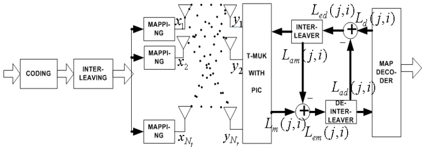
Figure 2.2: Structure of Turbo-MUK for single-user MIMO system

2.2.1

Detector stage

Detector stage in the turbo-MUK is build upon the MUK detector discussed in the preceding section. The main added features in the turbo-MUK detector stage are its ability to use soft information from the decoder stage to improve the detection process and to generate soft information at its output. Also, it incorporates par-allel interference cancellation, i.e., it tries to cancel out the interference from other streams while detecting a particular data stream. In the following discussion about the turbo-MUK detector stage we will stick to the system model used earlier (Section 2.1). The detection process starts with the application of the MUK algorithm on the pre-whitened received data block {Y_w(k)}_k=1,2,...,B, corresponding to the block of information bits transmitted. This gives an equalizer matrix W that can be applied on the received data to get an estimate for the block of transmitted symbols

Z(k) = WTY_w(k)

= GTX(k) +N_w(k), (2.24)

where G is the global response matrix. Its transpose is ideally (in a noise free envi-ronment) given by

GT =Π

        

ejφ1 _{0 . . . 0}

0 ejφ2 _{. . . 0}

..

. ... ... ... 0 . . . . . . ejφNt

         , (2.25)

place we can say that the estimated symbols for the kth transmitted sub-stream are Gaussian distributed and given by

z_j =µ_jx_k+η_j, (2.26)

whereµ_j = [GT_]

jk and ηj is a Gaussian random variable with zero mean and variance

υ_j2 = [Φ_Nw]_jj. z_j is the estimate for thekth transmitted symbol stream because of the ordering ambiguity inherent to blind detection. We can use the fact that estimated symbols have a Gaussian distribution to compute the soft information for the decoder stage in the following manner. Suppose each substream adopts M-ary quadrature amplitude modulation (M-QAM), then for each symbol intervalS_b =log₂M bits are jointly detected for each substream. The detector delivers the aposteriori LLR of the code bit b_j(i),1≤i≤S_b, j = 1, . . . , N_t

∧[b_j(i)] = logP[bj(i) = +1|zj] P[b_j(i) =−1|z_j] = logP[zj|bj(i) = +1]

P[z_j|b_j(i) = −1]+log

P[b_j(i) = +1]

P[b_j(i) = −1]. (2.27) The second term denoted by L_am(j, i) represents the apriori information about the code bit b_j(i) delivered by the decoder, whereas the first term denoted by L_em(j, i) represents the extrinsic information delivered by the detector. Since, z_j is Gaussian distributed, the probability distribution ofz_j given x_k is given by

P(z_j|x_k=x) = 1

(2πυ_j2)−1/2exp(

(z_j−µ_jx)2

2υ_j2 ). (2.28)

Denote X_j+ ={x_k =x :b_j(i) = +1} and X_j− = {x_k =x : b_j(i) =−1}, the extrinsic information delivered by the detector can be written as

L_em(j, i) = log

P

xk∈X_j+P[zj|xk]P[xk]/P[bj(i) = +1]

P

xk∈X_j−P[zj|xk]P[xk]/P[bj(i) =−1]

= log

P

xk∈X_j+exp(

(zj−µjx)2

2υ2 )Π1≤l≤Sb,l6=iP[bj(l)]

P

xk∈X_j−exp(

(zj−µjx)2

2υ2 )Π1≤l≤Sb,l6=iP[bj(l)]

, (2.29)

the extrinsic information generated for each substream is multiplexed into a single stream, de-interleaved and then fed to the decoder stage as apriori information L_ad. The decoder uses this soft information to generate apriori information for the detector (after interleaving and demultiplexing), which completes the first iteration of the signal estimation process.

The next iteration starts with computing the least square estimate for the channel matrix using soft information from the decoder

ˆ

H=YX˜H( ˜XX˜H)−1, (2.30)

where ˜X is the soft estimate for the transmitted signal vector. This soft information is also used to substract the interference signals from the received signal, which for some substream j gives

˜

Y_j = Y −HˆX˜_j

= HX−HˆX˜_j +N, (2.31)

where ˜X_j = [˜x₁, . . .x˜_j−1,x˜_j = 0,x˜_j+1, . . .x˜_Nt] is the estimated interference vector. Assuming near perfect interference cancellation (possible at high SNRs), now we can perform whitening operation as if there was only one transmitter. The pre-whitening transform is a 1×N_t row vector P_j obtained by taking the pseudo-inverse of the largest norm column of the matrix LD1/2, where L and D are computed by eigenvalue decomposition of the covariance matrix R_Y˜

jY˜j (see Section 2.1 for

defini-tions of L and D). Pre-whitening of the received signal obtained after interference cancellation gives an improved estimate for the signals in thejth _substream

z_j =P_jY˜_j. (2.32)

2.2.2

Decoder stage

The channel decoding stage of T-MUK uses the BCJR (L. R. Behl mar. 1974) decoding algorithm, which is better known for its ability to minimize probability of symbol error. However, the primary reason for selecting the BCJR algorithm (also known as the MAP algorithm) for the decoder stage here is the fact, that it can generate soft information in the form of log-likelihood ratios (LLRs) for the coded as well as the information bits, provided apriori LLRs for coded bits from the detection stage are available as inputs. In order to describe the functioning and main features of this algorithm we consider a binary 1/n convolutional code with the constraint lengthρ (decoding for turbo codes is similar). Also, we try to adhere to the notation used in the original paper wherever possible for clarity.

We start by assuming that the input to the encoder block at time t isI_t and the corresponding output isX_t= (x1_t, . . . , xn

t). The state of the encoder at time t is given

by

S_t= (s1_t, . . . sρ_t) = (I_t, . . . I_t−ρ+1). (2.33) The encoder starts in state S₀ = 0. An information sequence of input bits (length L) followed by ρ zero bits causes the encoder to end in state S_τ = 0, where τ = L+ρ. For convolutional codes this encoding process can be represented by a trellis structure. At the decoder, LLRs for coded bitsX_t= (x1_t, . . . , xn_t) and information bit I_tcorresponding to staget of the code trellis transiting from stateS_t−1 =s0 toS_t=s (where{x_j} ↔ {xk

t} withj = (t−1)n+k for a rate 1/n convolutional code) is given

by

∧(xk_t) = log

P

C_k+αt−1(s0)γt(s0, s)βt(s)

P

C−_k αt−1(s0)γt(s0, s)βt(s)

, (2.34)

where C_k+ is the set of state pairs (s0, s) such that the kth _{coded bit at stage t is 1}

and C_k− is the corresponding set for -1; and

∧(I_t) =log

P

I_k+αt−1(s0)γt(s0, s)βt(s)

P

I−_k αt−1(s0)γt(s0, s)βt(s)

, (2.35)

γ_t(s0, s) denotes the transition probability for the branch s0 →s for the staget of the code trellis and is given by

γ(s0, s) =P(S_t=s|S_t−1 =s0) =

n

Y

l=1

P(xl_t) =

n

Y

l=1

1

2[1 +xjtanh(λ

p

1(xj))], (2.36)

where {x_j} ↔ {xk_t} with j = (t−1)n+k, and λp₁(x_j) represents the corresponding apriori LLR delivered from the detector stage that is related to the state transition s0 →s. The other two terms, i.e.,α_t(s) and β_t(s) can be obtained by recursion as

α_t(s) =X

s0

α_t−1(s0)γ_t(s0, s), t = 1, . . . , τ, (2.37)

and

β_t(s) =X

s0

β_t+1(s0)γ_t+1(s0, s), t =τ −1, . . . ,0, (2.38) with boundary conditions given by

α₀(0) = 1, and α₀(s) = 0, f or s6= 0, (2.39) and

β_τ(0) = 1, and β_τ(s) = 0, f or s6= 0. (2.40) The summation of (2.37) and (2.38) are over all states s0 for which the transition s0 ↔ s is possible. Since, we are using this decoder in an iterative set-up, to avoid positive feedback (which may result in instability) we are more interested in comput-ing extrinsic information produced by the decoder given by

λ₂(xk_t) = log

P

C_k+αt−1(s0)βt(s)

Q_n

l=1,l6=kP(xlt)

P

C_k−αt−1(s0)βt(s)

Q_n

l=1,l6=kP(xlt)

= ∧₂(xk_t)−λp₁(xk_t), (2.41)

where∧₂(xk

t) is the LLR for coded bit computed in (2.34) and λp1(xkt) is the extrinsic

information for the coded bit delivered by detector stage.

(P. Robertson june 1995), where the computations are done in the logarithmic do-main can be used to solve the later problem. In addition Max-Log-MAP decoding reduces the computational complexity at the cost of a small loss in performance by considering only 2 trellis paths, the ML path and the closest path to the ML path as compared to the MAP algorithm which takes into account all the paths in the trellis. With the substitution of a_t = log(α_t), b_t = log(β_t) and c_t = log(γ_t), (2.34) can be rewritten as

∧(xk_t) = log(X

C_k+

exp(a_t−1+c_t+b_t)−log(X

C_k−

exp(a_t−1+c_t+b_t), (2.42)

where

c_t(s0, s) =

n

X

l=1

log(P(xl_t)) =

n

X

l=1

log( exp(x

l

tλp1(xlt))

1 +exp(xl

tλp1(xlt))

). (2.43)

The recursion equations to obtain a_t(s) andb_t(s) are given by

a_t(s) = log(X

s0

exp(a_t−1(s0) +c_t(s0, s))), (2.44)

with

a₀(0) = 0, and a₀(s) = −∞, f or s6= 0, (2.45) and

b_t(s) = log(X

s0

exp(b_t+1(s0) +c_t+1(s, s0))), (2.46)

with

b_τ(0) = 0, and b_τ(s) = −∞, f or s6= 0. (2.47) Using the approximation logP_iexi ≈ _max

| {z }

i

x_i, equations (2.42), (2.44), (2.46) be-come

∧(bk_t) =max_C+

k[(at−1+ct+bt)]−maxCk−[(at−1+ct+bt)], (2.48)

a_t(s) = max_{| {z }}

s0

[a_t−1(s0) +c_t(s0, s)], (2.49)

b_t(s) = max_{| {z }}

s0

[b_t+1(s0) +c_t+1(s, s0)], (2.50)

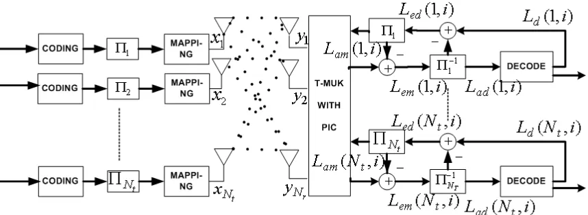
Figure 2.3: Structure of Turbo-MUK for multi-user MIMO system

2.3

Turbo-MUK for Multi-User MIMO

If we consider a number of users (sayN_t), with single antenna, transmitting inde-pendent data streams, and a receiver with multiple antennas (sayN_r), the whole set-up can be seen as anN_r×N_tdistributed MIMO system. If all the assumptions about the transmitted signals and the MIMO channel made in last section hold, then we can use the single-user T-MUK structure for blind multi-user detection, with some minor modifications, for jointly detecting signals transmitted from multiple users (transmit-ters). Figure 2.3 depicts the T-MUK structure for multiple users. The only difference from the single-user structure is that at the transmitter each substream (correspond-ing to a particular user) is encoded (convolutional or turbo cod(correspond-ing) independently. At the receiver, the MUK detector separates different signal streams and generates soft information as done earlier, but now instead of multiplexing and joint decoding, each signal stream has an independent decoder. Each of these decoders uses the soft information about a given stream from the detector and computes soft information (about the same stream) to be fed back to the detector.

signal streams, for the MUK criterion to be applicable, is that these streams should be i.i.d. In a multi-user scenario signal streams from different users can be assumed to be independent, also we can assume that all of them have zero mean (assuming all users implement same symmetric modulation scheme, such as 4-QAM), but different signal streams may have different power levels (variances). In the previous discussion about MUK algorithm we assume signal streams with equal power levels, here we show that the channel pre-whitening step of the MUK algorithm enables it to handle the unequal power case as well.

Ideally, estimated covariance matrix for the received signal is given by

ˆ

R_{Y Y} = HR_XXHH

= H         

σ₁2 . . . 0 0 σ₂2 . . .

..

. ... ... 0 . . . σ2_Nt

        

HH, (2.51)

whereσ₁2, σ2₂, . . . , σ2_Nt denote the variance (power level) ofN_tusers. Y, X andHdenote the received vector signal, transmitted vector signal and channel matrix respectively. Running eigenvalue decomposition on Rˆ_{Y Y} gives the decomposition Rˆ_{Y Y} = LDLH (see Section 2.1), where the non-zero part of the matrix LD1/2 is now given by

˜

L=HU

        

σ₁ . . . 0 0 σ₂ . . . ..

. ... ... 0 . . . σ_Nt

         , (2.52)

whereUis a unitary matrix and we construct ˜Las a matrix that containsN_tcolumns of LD1/2 with largest norms. We now pre-filter the received signal as

˜

where Pdenotes the pseudo-inverse of ˜L and is given by P=         

1/σ₁ . . . 0 0 1/σ₂ . . .

..

. ... ... 0 . . . 1/σ_Nt

        

U†H†, (2.54)

where † denotes pseudo-inverse. From (2.53) and (2.54) it is obvious that whitening removes the power inbalance from the input signal streams. Thus, pre-whitening effectively results in i.i.d. transmitted streams, which makes the MUK algorithm work for different users with unequal powers.

2.4

Numerical Results

In Sections 2.2 and 2.3 we have introduced T-MUK detection for single-user and multi-user MIMO systems. We now highlight the effectiveness of T-MUK through numerical results. In Section 2.2, while describing T-MUK we assumed that the receiver has phase and ordering information before it computes the soft information about the coded bits in the detector stage. However, an actual implementation of T-MUK will require the receiver to extract this information from the received signals. Therefore, we begin this section by listing the phase and ambiguity removal techniques we use in our simulations to obtain numerical results for T-MUK.

coded bits) computed by the decoder needs to be differentially encoded again, before being fed to the detector for next iteration. Now, if the decoder soft estimate about a particular bit is not reliable enough, the inherent structure of the differential encoder (any output bit depends on all previously fed input bits) results in an error propaga-tion to all subsequent bits. Thus, if we use differential encoding we cannot have an iterative information exchange between the detector and the decoder stages. In our simulations we use a very small training sequence (2 symbol periods) to remove the phase ambiguity (thereby making T-MUK a semi-blind MUD instead of completely blind MUD).

We simulate a N_r×N_t MIMO system, wherein each entry of the channel matrix H_Nr×Nt is chosen from a complex Gaussian distribution of zero mean and unit vari-ance h_ij ∼ N(0,1). Each substream employs a 4-QAM modulation and the coding scheme used is rate 1/3, 64 state convolutional code with generators (G₁, G₂, G₃) = [155,117,123]₈ (code proposed for EDGE). We transmit information in blocks of 384 bits over a quasi-static channel (i.e., channel stays in one state for one block and then changes to another value for next block and so on). We record the bit error probabil-ity of single-user T-MUK and multi-user T-MUK (users having unequal power levels) over a large number of data blocks.

The simulation results (BER vs SNR plots) for single-user T-MUK (6×4 MIMO system) are shown in Figure 2.4, from which we can see that first iteration of T-MUK detection gives a gain of more than 8dB as compared to the uncoded T-MUK detection at a BER of 10−3. Next few iterations, which involve parallel interference cancellation along with the exchange of soft information increase this gain by another

∼1.5dB. We can see that we require just 3 iterations to achieve convergence and get an improved estimate.

Figure 2.5 depict the simulation results for multi-user T-MUK (6 ×4 MIMO system), where all the users have different power levels and the power of the strongest user is 3db more than that of the weakest user. We can observe that T-MUK gives a gain of greater than 5db over uncoded MUK in the first iteration itself and another

4 6 8 10 12 14 16 18 20 22 10−3

10−2 10−1 100

Signal to Noise Ratio (in dB)

Bit Error Rate

Uncoded MUK T−MUK,1−iter,TL=2 T−MUK,2−iter,TL=2 T−MUK,3−iter,TL=2 T−MUK,4−iter,TL=2 T−MUK,4−iter,TL=4

4 6 8 10 12 14 16 18 20 22

10−3

10−2

10−1

100

Signal to Noise Ratio (in dB)

Bit Error Rate

Uncoded MUK T−MUK,1−iter,TL=2 T−MUK,2−iter,TL=2 T−MUK,3−iter,TL=2 T−MUK,4−iter,TL=2

2.5

Summary

Chapter 3

Semi-Blind interference

cancellation

3.1

Introduction

Figure 3.1: Multicell MIMO system (downlink). Each transmitter has N_t antennas and each receiver has N_r antennas

an interference-limited environment without any channel knowledge about the inter-ferers. The receiver structure proposed here employs T-BLAST (discussed later) to detect the desired signal and T-MUK to deal with inter-cell interference and iterates between the two in a group multistage fashion to further improve the performance.

3.2

Multicell MIMO System Model

In order to compare the performance of different MUD structures for a cellular system, we consider a multicell structure where each transmitter has N_t antennas and each receiver has N_r antennas. We take into account interference from the first tier of the center-excited cell configuration and assume a frequency-flat, quasi-static fading environment. The complex path loss between the jth _{transmit and the i}th

receive antenna is composed of three components, path loss (that depends on the link length and the path loss exponent), loss due to shadow fading and multipath fading loss. The baseband channel gain between a pair of transmit and receive antennas is modeled as

h_ij =

v u u t_c 1

dγ_ij

√

s_ij

 

s

R R+ 1e

iφij ₊ s

1 R+ 1mij



where d_ij is the length of the link, γ is the path loss exponent, c is the propagation constant, s_ij is the log-normal shadow fading variable, R is the Ricean factor, which denotes the ratio of the direct received power to the average scattered power, φ_ij is the phase shift of the direct path and m_ij is scattered component, modeled as a normalized Gaussian variable. In the following discussion, the model is further simplified by assuming absence of large obstacles and the LOS path, so that shadow-fading loss and the effect of Ricean factor on channel gain can be neglected.

In this study, the multicell MIMO system model is a straightforward extension of the single cell MIMO system model discussed in Chapter 2, and is given by

Y =HX+X

j

H_{if j}X_{if j} +N, (3.2)

whereX_{if j} denotes the transmitted signal from thejth interfering user, H_{if j} denotes the matrix capturing channel characteristics between the jth _{interfering user (in an}

adjacent cell) and the receiver in the cell of interest. The channel matrices H and

{H_{if j}}are mutually independent, with i.i.d. normalized complex Gaussian elements. The transmitted signals from the desired and interfering users are constrained to have a total transmit power of E[XH_{X] ≤ P and E[X}H

if jXif j] ≤ Pif j, respectively,

which includes the path loss factor. The noise is assumed to be white and circularly symmetric Gaussian with covariance Φ_N = σ2I. The signal to noise ratio (SNR) is given by ρ = P/σ2, and the signal to interference ratio (SIR) is given by η = P/P_jP_{if j}. The multicell system model discussed here is valid for the downlink as well as the uplink of a cellular system. Figure 3.1 depicts an exemplary cellular downlink scenario.

Figure 3.2: Multicell MIMO system model. Each interfering transmitter has a single antenna and each receiver has N_r antennas

3.3

Group Successive Interference Cancellation

In (Varanasi july 1995), the concept of group detection was introduced, where multiuser detection is performed in a sub-optimal fashion by jointly detecting a group or subset of all users. In simple terms group detection can be interpreted as a cascade of a decorrelator (for curbing the users outside the group) followed by an optimal detector for the users in the group of interest. Another interesting idea (Wyner jan. 1974) originally developed in the context of scalar-output Gaussian multiaccess channels, is that of successive interference cancellation (SIC). It involves decoding the users sequentially, that is, the first user is decoded by regarding interference from other users as noise. The decoded and re-encoded symbols of the first user are then subtracted from the received data and the second user is decoded by regarding the interference from remaining users as noise and so on. This strategy achieves the total capacity of Gaussian multiaccess channel.