Abstract— The convergence speed of the standard Least Mean Square adaptive array may be degraded in mobile communication environments. Different conventional variable step size LMS algorithms were proposed to enhance the convergence speed while maintaining low steady state error. In this paper, a new variable step LMS algorithm using the accumulated instantaneous error concept is proposed.
In the proposed algorithm, the accumulated instantaneous error is used to update the step size parameter of standard LMS is varied.
Simulation results show that the proposed algorithm is simpler and yields better performance than conventional variable step LMS.
Index Terms—Adaptive filters, adaptive array, variable step
LMS, moving object tracking.
I. INTRODUCTION
Adaptive beam former play an important rule in radar, sonar, speech processing and, more recently, in mobile wireless communications. It is desired to have a fast convergent adaptive antenna with good tracking capabilities of desired and interfering signals. This is to improve the user capacity for the base stations and the mobile handset in wireless communication system. Potential performance improvements for including interference reduction ,of moving sources, through adaptive beam forming motivates the development of fast convergent LMS algorithm.
As one may know, standard LMS is the most likely searching adaptive algorithm due to its simplicity, stability and performance prosperities. As a result many LMS based algorithms have been developed aiming to improve the convergence characteristics of the standard LMS. In the standard LMS, the step size is fixed and the filter weights are updated according to:
)
(
)
(
)
(
ˆ
)]
(
ˆ
)
(
)
(
)[
(
)
(
ˆ
)
1
(
ˆ
* *n
e
n
u
n
w
n
w
n
u
n
d
n
u
n
w
n
w
Hμ
μ
+
=
−
+
=
+
(1)It can be shown that the value of the step size parameter is fixed and governed by:
Manuscript received March 20, 2008.
Yu Gong, is with the Department of Electrical Engineering, University of Reading, Reading UK ([email protected])
Khaled F. Abusalem is with the Department of Electrical Engineering, University of Reading, Reading UK ([email protected]).
max
1
0
λ
μ
<
<
(2)Where
λ
max is the maximum eigenvalue of the underlying correlation matrix R.The standard LMS was simple, both in the number of calculations required for its update and its derivation from the method of steepest descent. Moreover it was robust in a number of applications. The adaptive feedback constant µ in the LMS controls the convergence rate of the filter coefficients, in addition to determination of the final excess error.
Since the convergence time is inversely proportional to µ, a large µ for fast convergence in tracking applications is always selected. However, large step size will result in increased misadjust met.
Hence, a set of LMS based algorithms known as variable step size algorithms were proposed to overcome this problem. In these algorithms the step size of the LMS is varied using different approaches. Among these variable step size LMS algorithms are the convex combinations of adaptive filters.
Recently, in H. Sayed and others CONVEX COMBINATIONS OF ADAPTIVE FILTERS, they used two independent filters with large and small step size. In their approach they used a mixing parameter to scale the output of both filters in order to combine advantages of both filters. The draw back of this algorithm is that they used two filters working in parallel. Moreover the MSE the switch over from the high step size to the small step size MSE in non smooth way. In their approach, the output of the filter is given by:
(3)
Where and are the outputs of two transversal filters at time n. The idea is that if is assigned appropriate values at each iteration, then the above combination will extract the best properties of filters
and .
This algorithm, however, introduce computational complexity as two different filters are used. Moreover, the mixing parameter, namely λ, is a function of the mean square error what means more filters need to work in
Variable Step LMS Algorithm Using the
Accumulated Instantaneous Error Concept
parallel to produce the mean value. In addition, the MSE does not converge smoothly to its final steady state value.
In this page, a new algorithm called accumulated instantaneous error driven LMS or AIED LMS is introduced which is utilizing the accumulated instantaneous error to control the step size µ. The way in which µ is changing depends only on the accumulated error. The advantage of using accumulated instantaneous error is that less complexity as only one filter is required. In addition, the transition from larger step size into smaller one is taking place smoothly, as will be seen from the results.
The AIED LMs provides good convergence characteristics with less complexity. It out performs standard LMS as well as convex combinations filters. The final section of this paper show simulation results for application of the algorithm in beam former.
II. THE AIED LMS ALGORITHM
The step size influences two important parameters, namely the MMSE (steady state behavior) and the convergence speed (transient behavior). As we have seen the step size is directly proportional to the convergence speed. However it is inversely proportional to the MMSE. What makes the compromise process difficult.
To overcome this problem, one can start with large step size, to enhance the convergence speed, and gradually (in jumping steps) reduce it to attain its minimum value, to achieve desirable MMSE. One should note that the step size should vary within the stability boundaries.
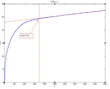
The way in which the step size is varied is very important. To achieve best performance the step size should jump to the next, smaller step, at the right moment. Having these jumps at the right moments will make the MSE converge smoothly and fast to the MMSE value. So the key factor for achieving this behavior is in the approach of selecting the break point for the MSE curve. By the break point we mean the point at which the MSE curve starts converging to its steady state, specifically the end of the transient portion of the curve as one can see from figure 1.
Smaller step size will result in a curve having its break point shifted from that of the larger step size, as one can see from the figure 1 above. So one can start with large step sizes and change over to the next, predetermined, step size at the instant when the MSE curve start bending (break point).
[image:2.612.311.526.70.237.2]Unfortunately doing the transition manually is not practical way of doing the transition from one step size to another. The MSE gradient is a good measure for the break point. Actually the gradient will be close to zero as the curve starts converging to the steady state values. Moreover the MSE is decreasing function of time and it fluctuates highly, due to the stochastic nature of the adaptive filter. Smoother MSE can be achieved but it needs ensemble averaging and as a result more complexity as parallel filters are required.
Fig. 1 MSE for 6 Elements Linear Array for Different Step Size Values
Fig. 2 AIE for 6 Elements Linear Array for fixed stp size
To overcome this problem we used the accumulated instantaneous error curve to identify the break point for smooth transition. The accumulated instantaneous means square error, abbreviated AISE here after, is always increasing function of time with minimum fluctuation as one can see from figure 2.
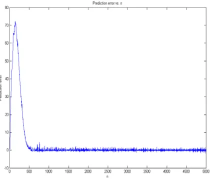
[image:2.612.308.528.287.465.2]Fig. 3 Prediction Error of AISE for 6 Elements Linear Array
To specify this break point we used a predictor. The predictor is a good tool for differentiating between curved and linear portions of the same curve. This is due to the fact that the prediction error will almost zero when the predictor work in the linear segment of the curve. The prediction error for the predictor is shown in figure 3. This figure shows that the prediction error for the AISE is even better to use to identify the break point for the transition from one step size to another smaller one. Actually the prediction error curve has two main linear segments with clear easy to find break point.
This break point can be identified by introducing a threshold such that when the prediction error decrease behind this threshold the algorithm will automatically transfer to the next smaller step size. A mathematical interpretation for the approach will be presented in the next few paragraphs.
III. MATHEMATICAL FORMULATION
The optimum filter weight vector
w
opt , Wiener optimum vector, is given by:xr xx opt
MMSE
w
R
r
w
=
=
−1(4)
Where R is the input correlation matrix and r is the cross correlation vector between the desired response and the filter input signal. Let the difference between the filter weight at time n and the optimal filter weight be given by:
v
n=
w
n−
w
opt (5) Then it can be shown that:n
n
I
R
v
v
+1=
(
−
2
μ
)
(6) Since R is positive definite, it has positive eignvalues. As a result it can be decomposed into an orthogonal matrix Q and an eigenvalue matrixΛ
as follows:Q
Q
R
=
TΛ
(7) Where)
,...,
,
(
0 1 −1=
Λ
diagonal
λ
λ
λ
M (8)Where
λ
m is themth
eigenvalue of R. Using equations above, it can be shown that the above equation can be written as:0
'
(
2
)
v
I
v
n=
−
μ
Λ
n (9) Where'
n
v
is a rotated version ofv
k by Q.A beamformer satisfying this equation is stable and convergent provided that the step size is with in boundaries given below:
max
1
0
λ
μ
p
p
(10)Where
λ
max is the largest eigenvalue of the correlation matrix R.The accumulated instantaneous mean squared error is the summation of individual instantaneous squared error values for different time instants. The AISE is given by:
2 1
(
(
))
)
(
n
e
i
AISM
=
∑
i=n (11) The above function is an increasing function of i. The function has an interesting characteristic over the MSE function. It can bee seen easily that the AISE curve behave in more tidy way than the MSE. It evolves smoothly with small fluctuation to its steady state value. One can differentiate between two main segments of the AISE curve. The first portion is the curved line where the gradient of the SISE starts from high values and converge to fixed steady state value. The other segment of the curve is linear at which the derivative is fixed.It is easier to manipulate the AISE than the standard MSE. This is due to the fact that the AISE has definite break pint which can be identified easily. Actually the break point is the point where the curve takes its linear behavior as reflected from figure 4 above.
To specify this break point we used a predictor. The predictor is a good tool for differentiating between curved and linear portions of the same curve. This is due to the fact that the prediction error will almost be zero when the predictor works in the linear segment of the curve. The prediction error for the predictor is shown in figure 3.
The predictor is an LMS filter in its own and has a pre determined order. The order of the predictor should be selected carefully to fit the job perfectly. It is better to keep the order as small as possible to improve the convergence proprieties having maximum of three taps.
In the proposed STVS-LMS algorithm, at every iteration time the prediction error, of the AISE predictor, is compared to a predetermined threshold. If the error is less than the threshold, the step size is changed to a smaller one. The process will proceed until the minimum step size is achieved. The proposed STVS-LMS is summarized below: Proposed STVS_LMS Algorithm
i. Decide order of the beam former M
ii. Decide initial step size
μ
n for n=1, the step sizedecrement and boundaries
iii. Decide the length (
M
p) of the predictor and its step size (μ
p)iv. Decide N, adoption course iteration numbers v. Decide the threshold for the smooth transition b. For n=1,2,3,…..N
i. Find instantaneous squared error, n
H n n
n
d
W
X
e
=
−
ii. Find accumulated instantaneous squared error, 2 1
(
(
))
)
(
n
e
n
AISM
=
∑
i=niii. Find prediction error for the AISM (PEAISM) iv. If PEAISM is less than threshold decrement the
step size v. Find new step size
vi. n
H n n
n
d
W
X
e
=
−
vii.
W
n+1=
W
n+
μ
ne
nX
nIV. SIMULATION RESULTS AND DISCUSSION
The simulated results for linear array will be presented in this section. The array parameters, inter-element separation and number of elements, will be fixed during the beam forming adoption course except for complex weights, amplitude and phase, of individual elements. The number of elements will be six and the inter-element separation will be fixed at
dx
=
0
.
5
λ
, where lambda is the wave length of theoperating frequency.
The proposed AIED-LMS algorithm is used to drive/steer the linear beam formers. The algorithm parameters will be determined for each scenario. These parameters include the step size decrement, predictor order, predictor step size, threshold among others will be given as the initialization parameters for the algorithm at the beginning of the adoption course.
In each scenario the number of interferers, co-channel interference, will be varied. Usually the number of interferers will be below that of the antenna/beam-former elements. The direction of arrival of different interferers and target will be varied too. Moreover different combination of target signal to interference and desired signal to noise ratios are applied to different scenarios.
The performance of the beam former and as a result the algorithm driving it will be tested for these scenarios with
many variables. Specifically the speed of convergence of the steering process for the main beam as well as nulls will be illustrated by performance measuring indices. These performance indices are mainly the mean square error and the array factor. Accumulated error and weight’s magnitude will be used when required.
In the simulation, a binary phased shift keying (BPSK) modulation scheme with a unit energy pulse was employed. The channel is assumed to be an AWGN channel. All displayed results have been averaged over two hundred independent runs.
In what follows, the proposed AIED algorithm performance will be highlighted in view of the below scenario. Simulation was run for a six elements linear array with inter-elements separation of half wave length. The channel is AWGN with SNR ratio of 10 dB and 0dB SIR. Both the desired and unwanted interferers are binary phase shift keying (BPSK) modulated with unity power. The angle of arrival for the desired signal is
θ
i=
0
, while that of the unwanted interferer is located atθ
i=
35
. The standard LMS was run for two different values of step size,μ
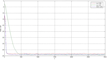
, which are .008 and .001. On the other hand a value which between 0.008 to .001 was selected for the AIED-LMS algorithms. The experiment has been run a two hundred independent times.At first it is important to see how the AIED-LMS out performs standard LMS as well as Convex Combinations in null steering capabilities. Figure 4 shows the MSE for AIED-LMS and that of the standard LMS for different step size values. As one can see the STVS converge faster with minimum steady state error. Actually the proposed algorithms combine convergence speed characteristics of LMS with large step size and at the same time steady state characteristics of the small step size LMS.
Similarly figure 5 shows the convex combinations versus the standard LMS for the same scenario. Comparing both figures one can easily see that AIED-LMS out performs both standard LMS as well as Convex Combinations. It converges fast and smoothly to its steady state values
V. CONCLUSION
The LMs is a simple and robust adaptive algorithm and has been used in variety of applications. Recently, more advance versions of the LMS have given significant improvements in convergence prosperities. However these algorithms introduced complexity to meet a satisfactory performance. A new algorithm, the AIED LMS, introduced the concept of accumulated instantaneous error to control the step size parameter.
Fig. 4 AIED versus LMS (µ=.001 and µ=.008)
Fig. 5 Convex combination versus LMS (µ=.001 and µ=.008)
REFRENCES
[1] S. Haykin, “Adaptive Filter Theory’’, Prentice Hall, fourth edition, 2001.
[2] C. A. Balanis, ‘‘Antenna Theory Analysis and Design’’, John Wiley, New York, second edition, 1997.