ISSN: 1992-8645 www.jatit.org E-ISSN: 1817-3195
CALIBRATION ALGORITHM FOR FREEHAND
ULTRASOUND
1
YAO RAO, 2YAO PENG 1
Aeronautic College, Shanghai University of Engineering Science, Shanghai 201620, China 2
School of Economics & Management, Beihua University, Jilin 132000, China
ABSTRACT
Ultrasound (US) image 3-D calibration for freehand probe is an extremely important technique in computerize 3-D ultrasonic (US image model reconstruction).Calibration is a procedure to calculate the spatial relationship between the US image and the tracker attached to the US probe. In this research, a different cross-string phantom and the corresponding algorithm are presented. The phantom with a set of crosses accelerates interactive operation speed through the strings and crosses out of the scanning plane guiding the operator quickly to find the scanning plane. The other, the ten crosses in the scanning plane provide the coordinates and spatial vectors for the calibration algorithm, thus the calibration algorithm can be optimized based on the least-squares fitting method of the homologous points matching. The results show that the scanning plane positioning time is no more than 5s. The precision and the accuracy demonstrate that the algorithm calculates more accurate matrix than that is obtained through other ways in the same operation time.
Keywords: Image Processing, Ultrasound Image Calibration, Homologous Points Matching
1. INTRODUCTION
To computerized reconstruct the three-dimensional (3-D) ultrasound solid model of the tumor, calibration for ultrasound (US) image is an obligatory procedure. When doctors hold the US probe, called freehand scanning style, to collect the image sequences, a series of non-parallel and irregular two-dimensional (2-D) ultrasound images are obtained. Current reconstruction algorithms and tookits, such as VTK (Visualization ToolKit), are all developed based on the regular parallel image sequences. So only these 2-D ultrasound images are transformed into 3-D space, and after pixel interpolation, can the regular and parallel image sequences be extracted. Then the 3-D reconstruction tookit will be feasible on tumor 3-D reconstruction. The above mathematical transformation procedure for 2-D coordinates of pixels in the US image to 3-D coordinates is the US image 3-D calibration. The core algorithm is calculating the transformation relationship between the US image and the tracking device attached to the US probe [8]. The transformation cannot be physically measured, only can be shown by a 4 × 4 matrix (rotation, translation and scale) through calculation.
The phantom, the speed and the precision are two important factors to evaluate the US calibration
method and algorithm [8]. From Detmer initially proposed a point target method and iterative least-squares fitting method to find the calibration matrix, the calibration researches on the phantom, the speed and the precision were uninterrupted. In the aspect of the calibration precision improvement, researchers have mainly focused on the optimization of the solid model with special geometric characteristics known (commonly be called phantom) to reduce the errors caused by interaction operations and calibration algorithms. Though the single point calibration method produced good results, it was time-consuming because it required collection of a large number of US images[8]. So in the last decade, to simplify the interaction and reduce the time, from Prager in 1998, Blackall in 2000, Pagoulatos and Muratore in 2001, Letotta in 2004, Sangita in 2005 to Hsu in 2008 [7], Abeysekera and De in 2011[2,3], Melvaer in 2012 [1], successively investigated their own optimized methods for phantoms and corresponding algorithms. To accelerate the calibration speed, Poon in 2005 [10], Hartov in 2010 [5], Hsu in 2008 [9], Chen in 2009-2011 [4,6], presented the real-time 3-D US calibration methods.
space vector was researched, which can optimize the least-squares fitting algorithm to calculate the more accurate calibration matrix than that is obtained through the other reported methods in the same operating time.
2. CALIBRATION METHOD
2.1 Theory of Calibration System
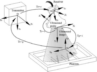
[image:2.612.92.300.320.474.2]The calibration is a procedure to find the spatial transformation relationships between the US image coordinate system and the tracking device coordinate system Tr←i. Current tracking sensors mainly include the magnetic tracker and the optical tracker. We selected the magnetic tracker which was also called magnetic receiver, receiver for short.
Figure 1: Coordinate Systems Definition And Transformation Relationships
The whole coordinate definition and transformation relationships of the calibration system are shown in Figure 1. Oi is the image coordinate system (this paper defined). Oris the magnetic receiver coordinate system (magnetic manufacturer defined). Ot is the magnetic transmitter coordinate system (magnetic manufacturer defined, as the 3-D spatial coordinate system in this paper). And the Tt←r is the transformation matrix that is the magnetic receiver coordinate system Or relative to magnetic transmitter coordinate system Ot. It is known from the algorithm of the magnetic tracking system. If an imaging pixel in the US image is marked as
[
0 1]
Ti h i v i
P = s ⋅x s ⋅y , sh ,sv are the image coefficients of the horizontal and the vertical directions (scales, mm/pixel), in general, sh=sv. it
can be transferred into the 3-D coordinate system Ot and be marked as Pt =
[
xt 0 1yt]
T . Thetransfer relationship is as equation (1).
0 1 1
t u i
t v i
t r r i t
x s x
y s y
T T
z ← ←
⋅
⋅
= ⋅ ⋅
(1)
Therefore, Tr←i is the research focus, and generally is calculated through a phantom with special geometric characteristics, see figure 1. Where Op is the phantom coordinate system (this paper defined). The calibration target is calculating the transformation matrix Tr←i between the Oi and
Or through the assistant coordinate systemsOt and Op. When the US probe is placed upon the phantom as seen in Figure 1, if a point in the
phantom is marked as Pp = xp yp 0 1T . The
coordinate transformation matrix between Op and Oi is:
0 1 1
p h i
p v i
p t t r r i p
x s x
y s y
T T T
z ← ← ←
⋅
⋅
= ⋅ ⋅ ⋅
(2)
Shortening:
p p t t r r i i
P =T ← ⋅T← ⋅T←P (3)
Where Tp←t is the transformation matrix between the magnetic transmitter coordinate system Otand the phantom coordinate system Op. It is calculated by the algorithm in this paper. Equation (4) is only by matrix expression:
p i p t t r r i
T ← =T ← ⋅T← ⋅T← (4)
Finally the image calibration Tr←i in matrix:
1 1
r i t r p t p i
T← =T←− ⋅T ←− ⋅T ← (5)
2.2 Phantom And Calibration
ISSN: 1992-8645 www.jatit.org E-ISSN: 1817-3195
dry and water conditions. The cotton stings pass through the holes, 1mm in diameter, on both front and back walls and form two layers of cotton strings arrays.
Figure 2: Phantom Construction And Coordinate Systems Definition
The 10 endpoints (holes) of all the vertical strings in the two sides opposite like in figure 2 are the marked points. They are marked as the stars, double 2 endpoints in the up side and double 3 endpoints in the down side. All coordinates of the marked points in the phantom coordinate system
p
P are given when the phantom is designed. Place the needle attached with the tracker (magnetic receiver) in the holes, through magnetic tracking algorithm Tt←r, the coordinates of these holes in
Ot (the magnetic transmitter coordinate system) are calculated, marked as Pt . Apply the least-square fitting to Pp and Pt:
2
,
min p ( t )
R p
∑
P − RP+p (6) Through finding the minimized distance between the homologous points Pp and Pt, the least-square fitting method calculate the transformation matrix( , ) p t
T ← = R p . Where R is rotation and p is translation vector [8].
2.3 Imaging
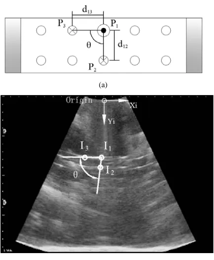
After phantom calibration Tp←t, place the US probe upon the cross-strings align with the middle string cross planar arrays like figure 3, adjust the probe’s orientation and position, to ensure the image plane make intersection with the cross-string layers. Until the 10 middle points are all in the US image, two layers, 5 imaging points in each layer, total 10 imaging points are shown. In this procedure, the strings trend nearby the middle cross arrays are help the probe find the middle cross arrays rapidly. The image origin is defined at the
[image:3.612.316.520.127.220.2]centre of the sector surface of the probe. See Figure 4.
Figure 3: Probe Scanning And Ultrasound Imaging
2.4 Image Calibration Algorithm
The image calibration algorithm is as in the figure 4. There are ten imaging points in the scanning image. They are the corresponding images of the cotton strings crosses in the phantom. But only two points’ coordinates are used in the calibration algorithm. They are I1 and I3, see the figure 4(b). The coordinates of P1, P2, P3, d12 and
23
d in the phantom are known by design, in figure
4(a)., so the angle θ between P P1 3 and P P1 2 is
calculated by P1 , P2 and P3. Then θ with the distancesd12 and d23 provide three parameters for calculating the image point I2 and I3 .
(a)
(b)
[image:3.612.90.301.150.266.2] [image:3.612.313.530.427.691.2]The calibration procedure is as followings: 1) Manual mark I1. I1is the middle point of the up layer of the ten points sequence in the scanning image. Select I1 as the datum point, because it is nearby the centre line of the sector region in the US image. As the datum of the other points, the distances of other points’ relative to it should be calculated. Its homologous point is the P1 in the phantom, homologous point in the receiver
1 r t t p 1
R =T← ⋅T← ⋅P.
2) Manual mark and calculate I2. I2is a point near the middle point of the layer below of the ten points sequence in the scanning image. Firstly, marking the highlight point below the datum point
1
I to determine the direction of the vector I I1 2 .
Then calculating the distance from I1 to I2 according to d12 (be converted to pixel). The homologous point of I3 is the P2 in the phantom. So homologous point in the receiver is
2 r t t p 2
R =T← ⋅T← ⋅P .
3) Calculate I3 . I3 is a point near the datum
point’ left side along the vector I I1 3. The direction
of I I1 3 is calculated by I I1 2 rotating an angle θ
around I1. And the distance from I1 to I3 can be calculated according to d13 (be converted to pixel). The homologous point of I3 is the P3 in the phantom. So homologous point in the receiver is
3 r t t p 3
R =T← ⋅T← ⋅P.
4) Repeat 1-3 in 4 different US images collected in one experiment.
5) Apply the least-square fitting to P Rr( ) and ( )
i
P I :
2 ,
min r ( i )
R p
∑
P − sRP+p (7)Where s is the coefficients of the image (scales, mm/pixel). Calculate the transformation matrix
( , ) r i
T← = R p (R : rotation matrix, p: translation vector) by the theory of finding the minimized distance between the homologous points Pr and
i
P[8]. Tr←i is shown as a 4 × 4 matrix (rotation, translation and scale) lile equation (9). Its first three columns form R and the fourth column forms p.
11 12 13 14
21 22 23 24
31 32 33 34
0 0 0 1 r i
P P P P
P P P P
T
P P P P
←
=
(8)
The calibration matrix can be calculated from a single US image. However, due to the variations in the whole operating procedure, the final calibration matrix is calculated based on 4 images repeated the manual marking and coordinates calculation. Then use each mass center of the homologous points to calculate the transformation matrix. In each US image, the imaging points are manual marked by our self-developed software.
3. EXPERIMENTS AND RESULTS
In our experiments, the devices were the ZK-3000 ultrasound equipment produced by Zhongke Tianli Ltd. in Beijing with the probe is 3.5/5.0 R60 and the AURORA magnetic tracker (attached to the probe) was from the NDI in Canada.
3.1 Calibration Precision
[image:4.612.104.515.598.715.2]The calibration precision can be evaluated by the discrete degree of the element in the calibration matrix [8]. The major factors causes the variations of the elements of calibration are: 1) Positioning errors when the stylus being placed into the hole on the phantom during phantom calibration (stylus
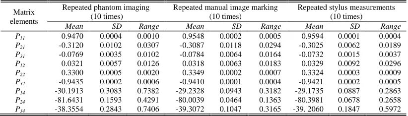
TABLE I: Precisions Statistics Of The Calibration Matrix Elements
Matrix elements
Repeated phantom imaging (10 times)
Repeated manual image marking (10 times)
Repeated stylus measurements (10 times)
Mean SD Range Mean SD Range Mean SD Range
P11 0.9470 0.0004 0.0010 0.9548 0.0002 0.0005 0.9594 0.0001 0.0004
P21 -0.3120 0.0102 0.0307 -0.3087 0.0118 0.0294 -0.3025 0.0062 0.0189
P31 -0.0769 0.0035 0.0102 -0.0784 0.0064 0.0164 -0.0732 0.0015 0.0037
P12 0.0321 0.0057 0.0126 0.0318 0.0063 0.0183 0.0329 0.0092 0.0296
P22 0.3300 0.0005 0.0020 0.3349 0.0002 0.0007 0.3324 0.0003 0.0009
P32 -0.9435 0.0002 0.0006 -0.9410 0.0001 0.0004 -0.9421 0.0002 0.0005
P14 -30.1913 0.3083 0.7382 -29.2328 0.0943 0.3182 -29.1735 0.0887 0.2863
P24 -81.6431 0.1593 0.4291 -80.0039 0.0464 0.1363 -80.3981 0.0678 0.2658
ISSN: 1992-8645 www.jatit.org E-ISSN: 1817-3195
measurements); 2) Placement incorrect when the phantom scanned by probe with freehand (phantom imaging); 3) Marking error of the pixel coordinates of the beads in the US image (manual image marking). Repeat each of above three operations 10 times and computing variations of the calibration matrix. The probe was moved away from the strings and repositioned for each of the 4 images. This method ensures the independency of each image collection and presents the actual precision of the repeated calibration. The results are shown in TABLE Ⅰ. The first six rows are the rotation matrix elements and the last three rows are the translation vector in millimeters. The third column of calibration matrix is not shown, because it is the cross-product of the first two columns. The maximum discrete degrees (0.4291mm-0.7406mm) are in the phantom imaging experiments. Compare this data with other past methods, such as 0.63mm-2.64mm (Letta reported in 2004), the calibration precision is improved.
[image:5.612.90.298.393.523.2]3.2 Reconstruction Accuracy
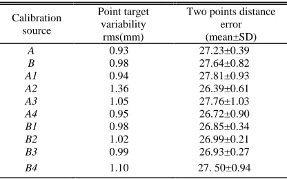
TABLE II: Comparison Reconstruction Results of Different Methods
The repeated precision reflects the stability degree of the calibration matrix, but does not provide an estimate of the validity of the calibration matrix, the effect of its 3-D transformation, so the reconstruction accuracy evaluation is necessary [8]. The method is: 1) Apply the calibration matrix to translate the ten points in each image into the 3-D coordinate system, and then calculate the root mean square (rms), evaluating the stability of reconstruction. 2) Apply the calibration matrix to translate the three point, I1, I2and I3, calculate the distance between I1 and I2 , I1 and I3 , then compare the distances with the real distances in the phantom. These data reflect the relative reconstruction accuracy. The results in TABLE II show that the reconstruction accuracy of the
multiple images calibration is higher than that of the single image calibration. The 3-D reconstruction accuracy is about ±1mm in both point target variability (repeated precision of reconstruction) and distance error (reconstruction accuracy). It is a relative high accuracy compare with other past researches.
4. CONCLUSION
This paper presents a different calibration method for freehand 3-D US system including cross-string phantom and corresponding calibration algorithm.
1) The phantom was made in a simple construction with common material. The ten crosses in the scanning plane provided the coordinates and space vectors for the calibration algorithm, and the crosses and the strings out of the scanning plane guided the probe to align with the scanning plane fast and accurately.
2) Based on the ten crosses coordinates, the space vectors and the angle between the two vectors were calculated, furthermore the homologous points in the US image and in the phantom were obtained, matching them through the least-squares fitting method to calculate the spatial transformation matrix between the US image and the tracking sensor attached to the US probe.
3) The scanning results show that the scanning plane positioning time is no more than 5s, faster than other method. And the precision and accuracy results demonstrate that the algorithm calculates more accurate calibration matrix than that is obtained through the past other published ways in the same operating time.
ACKNOWLEDGEMENTS
This work was supported by:
1) National Natural Science Foundation of China (30825010)
2) 2) Key Projects of Beijing Science & Technology committee (H060720050330).
REFRENCES:
[1] E. L. Melvaer, K. Morken, E. Samset, “A motion constrained cross-wire phantom for tracked 2D ultrasound calibration”, International Journal of Computer Assisted Radiology and Surgery, Vol. 7, No. 4, 2012, pp. 611-620.
Calibration source
Point target variability
rms(mm)
Two points distance error (mean±SD)
A 0.93 27.23±0.39
B 0.98 27.64±0.82
A1 0.94 27.81±0.93
A2 1.36 26.39±0.61
A3 1.05 27.76±1.03
A4 0.95 26.72±0.90
B1 0.98 26.85±0.34
B2 1.02 26.99±0.21
B3 0.99 26.93±0.27
[2] J. M. Abeysekera, R. Rohling, “Alignment and calibration of dual ultrasound transducers using a wedge phantom”, Ultrasound in Medicine and Biology, Vol. 37, No. 2, 2011, pp. 271-279. [3] D. De L, A. Vaccarella, G. Khreis, “Accurate calibration method for 3D freehand ultrasound probe using virtual plane”, Medical Physics, Vol. 38, No. 12, 2011, pp. 6710-6720.
[4] T. K. Chen, R. E. Ellis, P, “Abolmaesumi. improvement of freehand ultrasound calibration accuracy using the elevation beamwidth profile”, Ultrasound in Medicine and Biology, Vol. 37, No. 8, 2011, pp. 1314-1326.
[5] A. Hartov, K. Paulsen, S. Ji, “Adaptive spatial calibration of a 3D ultrasound system”, Medical Physics, Vol. 37, No. 5, 2010, pp. 2121-2130. [6] T. K. Chen, A. Thurston, R. Ellis, “A real-time
freehand ultrasound calibration system with automatic accuracy feedback and control”, Ultrasound in Medicine and Biology, Vol. 35, No. 1, 2009, pp. 79-93.
[7] P. Hsu, G. Treece, R. Prager, “Comparison of freehand 3-D ultrasound calibration techniques using a stylus”, Ultrasound in Medicine and Biology, Vol. 34, No. 10, 2008, pp. 1610-1621. [8] L. Mercier, T. Langø, F, Lindseth, “A review of
calibration techniques for freehand 3-D ultrasound systems”, Ultrasound in Medicine and Biology, Vol. 31, No. 4, 2005, pp. 143-165. [9] P. Hsu, R. Prager, A. Gee, “Real-time freehand
3D ultrasound calibration”, Ultrasound in Medicine and Biology, Vol. 34, No. 2, 2008, pp. 239-251.