Water demand forecasting using machine learning on weather and smart metering data

(1)

1

Water Demand Forecasting Using

Machine Learning on Weather and

Smart Metering Data

Submitted by Maria Xenochristou to the University of Exeter as a thesis for the degree of

Doctor of Philosophy in Water Informatics Engineering in September 2019

This thesis is available for Library use on the understanding that it is copyright material and that no quotation from the thesis may be published without proper

acknowledgement.

I certify that all material in this thesis which is not my own work has been identified and that no material has previously been submitted and approved for the award of a

degree by this or any other University.

(2)

2

Abstract

Water scarcity is a global threat due to lifestyle and climate changes, pollution of water resources, as well as a rapidly growing population. The UK water industry’s regulators demand plans from water companies to sustainably

manage their water resources, reduce per capita consumption and leakage, and create projections for climate change scenarios. This work addresses critical problems of water demand by expanding the understanding of water use and developing improved forecasting methods.

As part of this effort, the influence of the weather is thoroughly investigated, using a disaggregated, big-data statistical analysis. Results show that the weather effect on water consumption is overall limited, non-linear, and variable over time and households.

Next, a short-term demand forecasting model is developed, based on Random Forests, that predicts household consumption using several socio-economic, customer and temporal characteristics. This model is of significant value due to its accuracy as well as accompanying methodology that allows the

interpretation of results.

In order to further improve the forecasting accuracy achieved using Random Forests, a new modelling technique is developed. The new method that uses model stacking and bias correction, outperforms most other forecasting models, especially when past consumption data are not available, as well as for peak consumption days.

Finally, a water demand forecasting model based on Gradient Boosting

Machines is trained at different levels of spatial aggregation, for different input configurations. Results show that the spatial scale has a strong influence on the best model predictors and the maximum forecasting accuracy that can be achieved.

The methodology developed here can be used as a guide for researchers, water utilities and network operators to identify the methods, data and models to produce accurate water demand forecasts, based on the characteristics and limitations of the problem.

(3)

3

Acknowledgments

First and foremost I would like to thank my supervisor, Prof Zoran Kapelan for his continuous support, advice, motivation, faith, patience and assistance, every step along the way. Thank you for accepting me in this PhD program, for

enabling me to complete it on time and for always listening and helping me achieve my goals. And of course, thank you for your continuous input in this work, which shaped this thesis.

Next, I would like to thank my industrial collaborator, Dr Chris Hutton, for providing the data to make this project possible, as well as for his guidance, ideas and inspiration during our meetings and his input in this work. Thank you also goes to Prof Jan Hofman for his helpful comments.

I would also like to express my gratitude to Sebastian Gnann and Josh Myrans, who helped improve this thesis. Sebastian, thank you for your extremely

thoughtful comments, your time, effort and your ‘simple English’ approach. Josh, thank you for always answering my questions, for your wise words of wisdom and your helpful comments on this thesis. You both make academia the incredibly supportive, intellectually stimulating, friendly and kind place that I experienced it to be.

A big thank you to the Water Research Group at the University of Bristol, where I was hosted over the last 2 years. Even though a PhD can be a lonely path, my one has been quite the opposite, thanks to you. Many thanks to Prof Thorsten Wagener for his generosity, offering me to be part of this group that shaped my PhD experience for the very best. Special thank you to Elisa Bozzolan for being a great friend, colleague and supporter over these years.

Finally, thank you to my parents, for providing me with the education and opportunities in life to achieve my dreams and the upbringing to know it is possible.

(8)

8

List of Tables

Table 1.1. Types of urban water demand forecasts reported in the American Water Works Association water demand survey (adapted by Billings and Jones,

2008). ... 27

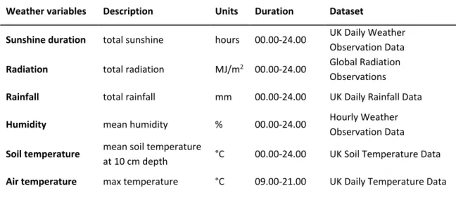
Table 2.1. Summary of the weather variables that are used in this study. ... 41

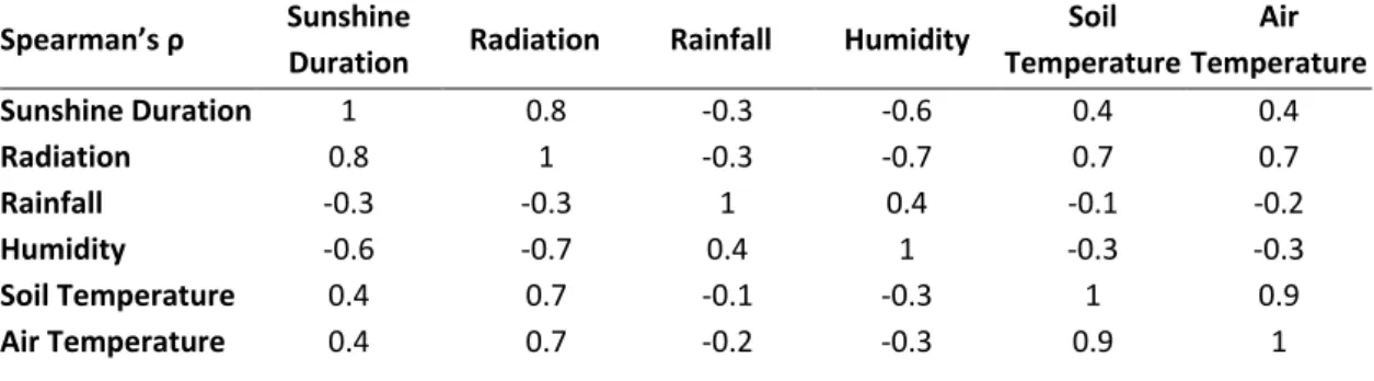
Table 2.2. Spearman’s ρ correlation coefficient for each pair of weather variables. ... 43

Table 2.3. Property segmentation of analysed consumption data. ... 44

Table 2.4. Customer segmentation of analysed consumption data. ... 44

Table 2.5. Temporal segmentation of analysed consumption data. ... 44

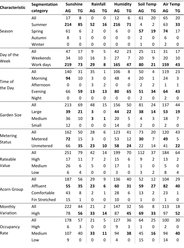
Table 2.6. Number of significant segments, i.e. the ones that have an absolute Spearman’s ρ correlation coefficient higher than |±0.5| at 99% confidence interval, for each category and weather variable (Sunshine duration, Rainfall, Humidity, Soil Temperature, Air Temperature), for all gradients (AG), as well as a gradient among the top 1/3 (TG)... ... 51

Table 3.1. Chi-square correlation statistic between each one of the six household variables. ... 69

Table 3.2. Input variables for Models 1-7. ... 76

Table 3.3. Model configuration and prediction accuracy for models 1-7 ... 83

Table 4.1. Input variables used to train each group of models. ... 97

Table 4.2. Hyperparameter values selected for the RF model, for Groups 1 and 2. ... 108

Table 4.3. Hyperparameter values selected for the GBM model, for Groups 1 and 2. ... 108

Table 4.4. Hyperparameter values selected for the XGBoost model, for Groups 1 and 2. ... 108

Table 4.5. Hyperparameter values selected for the ANN model, for Groups 1 and 2. ... 108

Table 4.6. Hyperparameter values selected for the GLM model, for Groups 1 and 2. ... 108

Table 4.7. Hyperparameter values selected for the DNN model, for Groups 1 and 2. ... 108

(9)

9

Table 4.8. Model comparison (a) with and (b) without past consumption as input, for the test dataset, for seven model types and four bias correction

methods. ... 110 Table 5.1. Categories formed for each household characteristic. ... 122 Table 5.2. Model configurations tested at each level of spatial aggregation. . 126 Table 5.3. Prediction accuracy for nine models, trained on different household groups. ... 129 Table 5.4. Household group sizes, number of data points and daily water

consumption range, for each spatial aggregation level ... 131 Table 5.5. MAPE for eight model configurations, for predictions one and seven days into the future, for three spatial aggregations of properties (network, areas, districts). ... 133

(10)

10

List of Figures

Figure 1.1. Household water demand forecasting best practice (adapted by UKWIR, 2015). ... 29 Figure 1.2. Overview of the thesis structure and the main topics that are

addressed in each chapter. ... 32 Figure 2.1. Distribution of correlation coefficients and gradients for segments that correspond to various combinations of weather variables and other

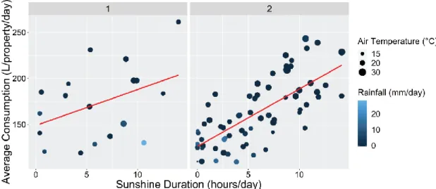
characteristics (household, customer, temporal). Each point demonstrates the correlation coefficient and gradient for the relationship between consumption and a weather variable, for one segmentation of consumption. ... 48 Figure 2.2. Correlation between total sunshine hours (hours/day) and average daily consumption (averaged across all properties), for summer evenings and affluent residents with high variation in their monthly consumption, in unmetered properties, during (1) weekends and (2) working days. ... 53 Figure 2.3. Correlation between total rainfall (mm/day) and average daily

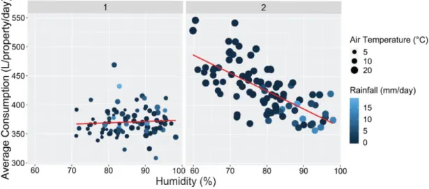
consumption (averaged across all properties), for (1) all properties and days, and (2) properties with affluent residents with high variation in their monthly consumption, in unmetered properties, during summer, working days. ... 54 Figure 2.4. Correlation between humidity (%) and average daily consumption (averaged across all properties), for working days and customers with high variation in their monthly consumption, in unmetered properties with high

rateable value, during (1) winter and (2) summer months. ... 54 Figure 2.5. Correlation between soil temperature (°C) and average daily

consumption (averaged across all properties), for working days and affluent residents with high variation in their monthly consumption, in (1) metered and (2) unmetered properties. ... 55 Figure 2.6. Correlation between air temperature (°C) and average daily

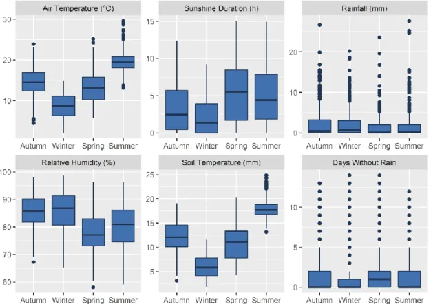
consumption (averaged across all properties), for working days and customers with high variation in their monthly consumption, in unmetered properties with (1) financially stretched and (2) affluent residents. ... 56 Figure 3.1. Variation of six weather variables within each season over the study period. ... 70 Figure 3.2. Distribution of consumption for different categories of six household characteristics. Each distribution comprises of mean daily consumption,

(11)

11

aggregated among all properties with the corresponding characteristic, for each day in the data. ... 77 Figure 3.3. Distribution of consumption for different categories of temporal characteristics. Each distribution comprises of mean daily consumption, aggregated among all properties for each day in the data, for different (a)

weekdays, (b) months, (c) seasons and (d) day types. ... 78 Figure 3.4 Contour plot for the MSE of the validation dataset when (a) all

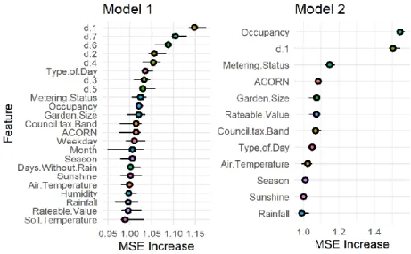
variables including past consumption are included in the model and (b) when past consumption data is not available. The crosses correspond to the point in the grid with the lowest MSE. ... 79 Figure 3.5. Factor by which the MSE increases when each feature is

permutated for models 1 and 2. ... 81 Figure 3.6. Factor by which the MSE increases when each feature is

permutated for models 3 - 5. ... 82 Figure 3.7. Influence of six household characteristics on predicted water

consumption - ALE plots. ... 84 Figure 3.8. Influence of four temporal characteristics on predicted water

consumption - ALE plots. ... 85 Figure 3.9. Influence of four weather variables on predicted water consumption – ICE plots. ... 86 Figure 4.1. Location of property areas (red) and weather stations (blue). ... 96 Figure 4.2. Metered against predicted values for (a) the GLM and (b) the

stacked-BC2 model, without past consumption as input. ... 111 Figure 5.1. (a) Range of household group sizes for each level of spatial

aggregation, among different days and groups. (b) Spatial scales created using the level of spatial aggregation and a fixed group size, varying from 5

households for the district level to 600 for the network level. Each disc illustrates the size and number of groups for one day in the data ... 124 Figure 5.2. Model accuracy (MAPE) for each household group size, for the test dataset. ... 130 Figure 5.3. Mean Absolute Percentage Error (MAPE) for different model

configurations (models 1-8) and different spatial aggregations (network, areas, districts), for all days in the data (plots a-c), as well as peak days (plots d-f)..132

(12)

12

Author's declaration

This thesis is presented as a collection of four journal papers that have been published or have been submitted for publication to academic journals. Each one of the papers forms one chapter of this thesis (see chapters 2-5).

Modifications have been made to improve consistency throughout the thesis. All papers have been written by the author and have benefitted from the comments of the co-authors. An explicit statement at the beginning of each chapter states the citation of the paper it corresponds to as well as the contributions of the author and co-authors of the paper.

(13)

13

Definitions

Property Characteristic: Customer Characteristic: Household Characteristic: Temporal Characteristic: Weather Characteristics: Variable: Segment:

An attribute of the properties in the dataset. It can refer to the garden size, rateable value, council tax band, or metering status of a property.

An attribute of the customers in the dataset. It can refer to the acorn group, occupancy rate, or

consumer behaviour (variations in average monthly consumption).

A property or customer characteristic.

An attribute that relates to time. It can refer to the time of day, the type of day (working day or weekend/holiday), the month, or the season.

An attribute that relates to weather. It can refer to air temperature, soil temperature, humidity,

sunshine duration, radiation, rainfall, or number of days without rain.

A household, temporal, or weather characteristic can be used as a variable in the analysis. The terms variable and characteristic are often used interchangeably in the text.

A homogenous group of consumption or

households. All components of a segment share the same household and temporal characteristics (e.g. the same garden size).

(14)

14 Segmentation:

Segmentation Category:

The process of creating consumption or household segments.

A type of consumption or household that has a certain temporal or household characteristic. One segmentation category includes all consumption or household segments that share the same

(15)

15

List of Abbreviations

Acorn ALE ANN BC DMA DNN GBM GLM ICE MAE MAPE MIDAS MSE Ofwat PCC PDP RF UKWIR XGBoost XRT

A Classification Of Residential Neighbourhoods Accumulated Local Effects

Artificial Neural Network Bias Correction

District Metered Area Deep Neural Network Gradient Boosting Machine Generalised Linear Model

Individual Conditional Expectations Mean Absolute Error

Mean Absolute Percentage Error

Met Office Integrated Data Archive System Mean Square Error

Office of Water Services Per Capita Consumption Partial Dependence Plot Random Forest

UK Water Industry Research Extreme Gradient Boosting Extremely Randomised Trees

(16)

16

1.

Introduction

1.1.

Motivation

Water is essential for the survival of humans, the preservation of the natural environment, the function of societies, as well as the operation of industry and agriculture. However, water is also a limited resource, threatened by

environmental changes and societal reforms, urbanisation, population and business growth, as well as the pollution of water resources.

The UK water industry, privatised in 1989, aims to provide clean water to its customers for four distinguished uses: urban, power generation, industrial and agricultural (Butler and Memon, 2006). Urban water use accounts for the water that is provided to residents (residential demand), businesses (commercial demand) and other organisations within a community or urban area (Billings and Jones, 2008).

The major droughts of 1975/76, as well as the subsequent droughts in the 1990s saw the UK imposing water restrictions and highlighted the vulnerability of the country’s water security to weather and climate changes (Parker and Wilby, 2013). Since then, the water industry’s regulators have consistently included requirements for assessing potential climate change impacts on the water supply (Beran and Arnell, 1989; Defra, 2003; Downing et al., 2003;

INTRODUCTION

(17)

17

Environment Agency, 2003) and later also for adaptation plans (The UK Government, 2008).

Given the risks to the UK water security, the full extent of the benefits, potentials and limitations of water management need to be well understood and the

heterogeneity of water use behaviours taken into account (Parker and Wilby, 2013). Emerging technologies and increases in computing power provide new ways to process large quantities of data in parallel and in reasonable time, which allows extracting values, causes or events from historical data that might have been overlooked in the past (Garcia et al., 2015). This information can be used to develop credible water demand forecasts, as well as pro-active

strategies that can assist with optimising network operations and building network resilience.

However, understanding and modelling water demand involves the consideration of a variety of factors such as lifestyle changes, household formation, population growth and weather characteristics, in order to ensure a trustworthy projection for the future. This work uses smart demand metering data, household characteristics and weather variables to gain a better

understanding of water demand and its influencing factors, as well as develop an improved water demand forecasting methodology.

The rest of this chapter provides the necessary background information and sets the terms and concepts that are going to be discussed in this thesis. It starts with describing the main aspects of water use and the concept of water demand forecasting, in terms of its characteristics and best-practice approach. Next, the key research questions and objectives of this work are introduced, followed by an outline of the thesis. Finally, a list of available resources,

including links to publications and code, are provided at the end of the chapter.

1.2.

Background

According to Billings and Jones (2008), urban water demand forecasting is ‘the process of making predictions about future water use based on knowledge of historical water use patterns’.

(18)

18

1.2.1.

What is water demand?

As part of this work, the first question that needs to be answered is ‘what is water demand?’. Some studies (Bellfield, 2001; Merrett, 2004; Rinaudo, 2015) define water demand as the water required by customers for various uses, such as domestic, industrial or agricultural. Another interpretation (Billings and Jones, 2008) defines water demand as ‘the total volume of water necessary or needed to supply customers within a certain period of time’, including leakage and all other inevitable water losses. In this thesis, the terms water demand, water use and water consumption are used interchangeably to refer to the total amount of water used by customers. This includes water losses on the customer side but excludes the associated water losses within the network (e.g. due to leakage or fraudulent abstractions).

1.2.2.

Water demand metering

Traditionally, residential water demand in the UK is not billed based on meter readings. Unmetered customers are charged a fixed amount per year instead, dependent on property characteristics such as the number of bedrooms, type of property, number of occupants or a company average. This is further adjusted according to the property’s rateable value, which reflects the rental value of the property and was last updated in the 1970s (Defra, 2008).

Water metering is part of a new, sustainable, environmentally friendly policy that aims to reduce water demand and secure water supply now and in the future. A water meter (similar to a gas or electric meter) is a device that measures how much water is used. Typically, water meters are read twice per year (Ofwat, 2013). Water metering is regarded as the fairest way to charge customers, since it requires them to pay for the volume of water they have used.

Historically, most properties in the UK have paid a standard, flat rate for their water use, regardless of actual consumption. However, water companies forecast that more than half of the homes in the UK will be on a meter by 2020 (CIWEM, 2015).

Unlike conventional metering devices, smart meters can record consumption in regular, much more frequent time intervals (e.g. every 15/30 minutes or even a handful of seconds) and are able to communicate that information wirelessly.

(19)

19

Thus, they can provide descriptive statistics (e.g. flow rates) as well as a better understanding of consumption (Pericli and Jenkins, 2015). Potential

applications of smart demand data include leak detection and variable water pricing, as well as improved network operations and demand forecasting (McKenna et al., 2014).

1.2.3.

Water demand modelling

Water demand modelling can be used for many purposes, such as demand pattern recognition and forecasting, user profiling, as well as identifying the determinants of water consumption.

According to Cominola et al. (2015), the existing literature can be divided into two distinct types, descriptive and predictive studies. Descriptive studies are useful for the analysis of patterns in the data that can improve the

understanding of when, where, and why water is used. Predictive studies focus on predicting future demands. Machine learning methods have been employed in the literature for both descriptive and predictive purposes.

More details regarding the types of models and methods that are used in each case are provided in the following.

1.2.3.1.

Machine learning models

Machine learning is the process through which machines or computers learn how to perform a task, using data. As machine learning becomes increasingly popular and algorithms become more sophisticated, machine learning based methods have dominated the recent demand forecasting literature. Although they have been so far primarily used for predictions, machine learning methods can find useful applications in descriptive studies. This is facilitated further by the data availability, new techniques, and computing power, which have not been available in the past.

Machine learning techniques can be divided in supervised learning, unsupervised learning, and reinforcement learning. Supervised learning

includes prediction tasks where the outcome is known and the algorithm learns to make predictions on new data (Molnar, 2019a). Examples of supervised learning algorithms are Artificial Neural Networks, Random Forests, and

(20)

20

the outcome is unknown (Molnar, 2019a). The task in this case is to identify common features and create clusters of data points (Antunes et al., 2018). Finally, in reinforcement learning the machine creates the dataset by running examples and evaluating the results (Antunes et al., 2018), with the aim to maximise a reward.

Both supervised and unsupervised learning are used within this thesis, although all forecasting models are based on supervised learning methods. Detailed information about the machine learning techniques used in each chapter are provided within the methodology section of the corresponding chapter. A detailed review of the studies that have used these methods for water demand forecasting tasks is also available within the literature review section of each chapter.

A major disadvantage of machine learning methods is their level of interpretability, i.e. understanding how the model makes predictions, as machine learning models are often considered ‘black box’. This name implies that information comes inside the box and predictions come out of the box but there is no understanding or knowledge of what is happening inside it.

Interpretability should be an important aspect of developing machine learning models, as it is a way to enhance the understanding of a process and ensure the model performs well by sanity checking the results.

Although interpretable machine learning is a relatively new field, few studies developed methods that enable the modeller to peek inside the black box and make conclusions on the role of the input data in making predictions (Goldstein et al., 2015; Apley and Zhu, 2016; Zhao and Hastie, 2018; Fisher et al., 2019; Molnar, 2019). The idea behind many interpretability techniques is to assess how the model predictions change, in terms of accuracy and direction, i.e. whether they increase or decrease, for a change in one or more input variables. A detailed description of the specific interpretability methods used in this study are provided in chapter 3.

1.2.3.2.

Descriptive models

The purpose of descriptive studies is to analyse consumption in order to make conclusions regarding the water use of different types of customers, identify the drivers of water demand, as well as explore patterns in the data. The results of

(21)

21

this analysis can be used to enhance the understanding of water demand and develop improved demand management strategies.

Typically, descriptive studies (Domene and Sauri, 2005; Babel et al., 2007; Schleich and Hillenbrand, 2008; House-Peters et al., 2010; Chang et al., 2010; Hussien et al., 2016) use simple statistical techniques in order to assess the relationship between consumption and a variety of property, customer, temporal, and weather characteristics. In some cases, machine learning or visual methods have also been employed to identify patterns in water demand or cluster consumption and group households based on their consumption behaviour.

A very common technique used to analyse and gain a better understanding of the dataset is to use descriptive statistics (Domene and Sauri, 2006; House-Peters et al., 2010; Pullinger et al., 2013). These methods are used to provide an overview of the dataset by using measures such as the mean or the variance of a population and demonstrate the frequency of occurrence of a characteristic. Another very common technique uses econometric and statistical models, such as multiple linear, piecewise, and polynomial regression (Domene and Sauri, 2006; House-Peters et al. 2010; Chang et al., 2010; Hussien et al., 2016) or log-log and semi-log-log models (Schleich and Hillenbrand, 2008) to investigate the influence of several demographic, behavioural, economic, and environmental factors on water use. These models are popular due to the fact that they are easy to use and interpret.

Other studies estimate the relationship between a variety of influencing factors and water use by assessing the strength of the correlation between them, using the value of a correlation coefficient (Babel et al., 2007; Chang et al., 2010; Hussien et al., 2016). This is a simple approach, although it does not account for the interactions between the variables or the temporal and spatial variation of the effect on water consumption. Methods such as data disaggregation can be useful in accounting for these interactions.

Finally, in some cases, methods such as clustering and data visualisations can offer additional information that would otherwise be very difficult to identify. Clustering methods have been used to find consumption patterns and groups of households with similar consumption behaviour (Pullinger et al., 2013), whereas

(22)

22

visual methods can be useful in identifying spatial trends (House-Peters et al., 2010; Chang et al., 2010).

1.2.3.3.

Predictive models

There are several water demand forecasting approaches and the most appropriate one needs to be selected with respect to the specific aim, forecasting objective, time horizon, as well as availability and resolution (time and spatial) of the available dataset. One way to group water demand forecasting models is based on their input data and model structure. According to this, they can be classified into micro-component studies, time series analysis, statistical, artificial intelligence, and hybrid models.

In micro-component analysis, ownership level, frequency of use, and volume per use of household appliances, as well as peak use hours, are taken into consideration (Butler and Memon, 2006). Several studies tried to identify patterns and trends using household micro-components (Butler, 1993; Edwards and Martin, 1995; Gurung et al., 2014). However, disaggregating water use requires large amount of data from different sectors, or very high resolution smart demand metering data, that are not typically available. According to the UK Water Industry Research (UKWIR) household consumption forecasting guidance manual, guidance for previous water resources management plans recommended micro-component analysis as the favoured method. However, in the most recent one it was regarded as too data intensive and complex (UKWIR, 2015). In addition, concerns regarding energy spending and carbon emissions (Fidar et al., 2010) also contribute to making micro-component modelling an unattractive option. Time series models (Froukh, 2001; Kofinas et al., 2014; Brentan et al., 2017; Chen and Boccelli, 2018) are based on the assumption that future trends in water use can be predicted based on historical water use (Billings and Jones, 2008). These models are often used for real-time forecasting and online applications. The Auto-Regressive Integrated Moving Average (ARIMA) method is one of the most important and widely used linear models in time series forecasting, as it has the ability to capture general trends and seasonal variations. The Holt-Winters method is a simple, exponential smoothing method applicable when the time series contain a seasonal component. It is a standard method used for automatic forecasting (Quevedo et al., 2014) and works best when the seasonal variations

(23)

23

are roughly constant throughout the series (Kofinas et al., 2014). Although they are quick to train, as well as simple and easy to use, time series models do not typically account for several other variables such as household and customer characteristics that also have an effect on consumption.

Statistical models (Herrington, 1996; Downing et al., 2003; Firat et al., 2009; Haque et al., 2014; Bakker et al., 2014; Fontanazza et al., 2014) consider a variety of variables and estimate statistically historical relationships between dependent and independent variables. This method is very common in the literature, since it integrates the effect of socio-economic and climatic factors, as well as public water policies and strategies. Therefore, it provides water operators with insights regarding the influence of different variables on water use. This is the reason that these models are also frequently used in descriptive studies, where forecasting is not the main goal.

Machine learning algorithms (Froukh, 2001; Cutore et al., 2008; Firat et al., 2009; Bai et al., 2014; Bakker et al., 2014; Romano and Kapelan, 2014; Shabani et al., 2016) have been proven effective to predict short-term, medium-term, and long-term water demand. Artificial Neural Network (ANN) based models are some of the most commonly used machine learning techniques in water demand forecasting and are often suggested as the best in the literature. The downside of these methods is that they are considered ‘black-box’, hence results obtained this way are harder to interpret. This means that although they can achieve high accuracy, their results cannot be used directly to shape demand management strategies and planning.

Finally, hybrid models (Bakker et al., 2014; Anele et al., 2017) have the

advantage of combining different model capabilities, focusing on emphasising positive and reducing negative capabilities of individual models (Kofinas et al., 2014). However, these models can also be hard to interpret as they make predictions by combining the results of individual learners, thus they lack any model structure.

Machine learning and hybrid models are used in this study for their accuracy as well as ability to capture complicated relationships between several predictors. In addition, the use of several interpretability methods allows to use these models not only in order to produce accurate demand forecasts but also in

(24)

24

order to gain an improved understanding of the factors that influence water consumption.

1.2.3.4.

Model assessment

An essential step of every forecasting methodology is the model assessment, i.e. the process of determining how well the model performed. This is a fairly abstract definition, as it depends on the objective and characteristics of the study. For example, a model might have a very good overall accuracy but perform poorly on peak consumption days, which are of high importance to water utilities. On the other hand, even if the model has a good accuracy for all days, it could be hard to interpret and therefore it might have limited use for operators.

When it comes to water demand forecasting, there is no acceptable level of accuracy pre-defined by the UK water regulators. The cost-benefit of improving forecasts should be considered and the favoured methodology should be determined based on the circumstances. For water scarce areas that are in danger of not being able to fulfil the supply-demand balance, achieving a high accuracy is essential in order to provide guidance and mitigate risks (UKWIR, 2015). However, when potential prediction errors do not threaten the system’s capacity to supply water to customers, less costly and sophisticated models can be considered as good alternatives.

In many cases, factors such as the model complexity and training time as well as data requirements might limit the applicability of a model in real-life

problems. Thus, the modelling technique needs to be selected based on the appropriate metrics that evaluate its performance with respect to the needs of the case study, while accounting for the requirements and limitations of its application.

Some metrics that are used frequently in the literature appear in the following, where nis the total number of values,

O

iand

P

iare the

i

thobserved and

predicted values, and

𝑂̂

and

𝑃̂

are the observed and predicted means, respectively:

(25)

25

 The Root Mean Square Error – RMSE (Dos Santos and Pereira, 2014; Kofinas et al., 2014; Shabani et al., 2016; Tiwari et al., 2016) is the square root of the Mean Square Error - MSE and is expressed as

RMSE

=

√

1

𝑛

∑

(𝑂

𝑖

− 𝑃

𝑖

)

2 𝑛

𝑖=1

= √𝑀𝑆𝐸

The RMSE is a measure of overall performance although it is sensitive to larger errors (Tiwari et al., 2016).

 The coefficient of determination - R2_{(Babel et al., 2007; Bakker et al.,}

2014; Dos Santos and Pereira, 2014; Haque et al., 2014; Kofinas et al., 2014; Shabani et al., 2016; Tiwari et al., 2016) is expressed as

R

2

=

[

∑ (𝑂𝑖−𝑂̂ 𝑛 𝑖=1 )(𝑃𝑖−𝑃̂) √∑𝑛_𝑖=1(𝑂_𝑖−𝑂̂)2∑𝑛_𝑖=1(𝑃_𝑖−𝑃̂)2

]

2

The R2_{values vary from 0 to 1 and indicate the degree of correlation}

between modelled and observed values (Haque et al., 2014).

 The Mean Absolute Percentage Error – MAPE (Bai et al., 2014; Kofinas et al., 2014; Candelieri et al., 2015; Tiwari et al., 2016) is expressed as

MAPE =

100 𝑛

∑

|

𝑂_𝑖−𝑃_𝑖 𝑂_𝑖 𝑛 𝑖=1

|

The advantage of the MAPE is that it is independent of units and therefore system capacity, which means it can be used to compare results from different studies and utilities (Candelieri et al., 2015).



The

Mean Absolute Error – MAE (Herrera et al., 2010; Dos Santos and Pereira, 2014; Kofinas et al., 2014; Shabani et al., 2016; Antunes et al., 2018) is expressed as

MAE =

1

𝑛

∑

|𝑂

𝑖

𝑛

𝑖=1

- 𝑃

𝑖

|

The MAE does not assign a higher importance to larger or smaller errors, nor does it take into account the sign of the error. It is merely an

indication of the overall agreement between predicted and observed values (Tiwari et al., 2016).

(26)

26

The above performance metrics constitute some commonly cited statistical tests, however, another validation method might be fit for purpose, depending on the respective forecasting aim. Since the selection of the assessment metric could determine the results and conclusions of the study, it is important that this is chosen with respect to the individual aspects of the problem and the research question.

1.2.4.

Water demand forecasting

1.2.3.1.

Forecast variables

Household water demand can be explored at different temporal and spatial scales, depending on the available data and tools, the selected methodology and the purpose of use. Water demand can be linked to individuals or be aggregated at the household and area level or even across the whole supply zone. It can reflect average annual, monthly, daily or hourly water use, while with the advent of smart demand meters, it can even go down to a few seconds. Typical end-use studies report per capita consumption (PCC) or per household consumption (PHC) (Gurung et al., 2014).Demand that is analysed at ‘per capita’ or ‘per household’ level is then multiplied by the total population or properties (UKWIR, 2015), in order to determine total demand. PCC can be calculated separately for metered and unmetered customers, as well as for different groups, based on the selected variables or clustering methods. According to Waterwise (2019), the average PCC in England is 150

litres/person/day, although the target is to reduce it to 130 litres/person/day by 2030 (Defra, 2008).

An example of the various types of forecast variables, along with their popularity among water utilities, is provided in Table 1.1. The data was obtained from 662 North American water supply systems, on a volunteering basis, and was

published in the American Water Works Association (AWWA) water demand survey (Billings and Jones, 2008). Overall, predictions of hourly and peak demands are useful in managing the network and ensuring sufficient water supply, while seasonal and annual predictions are used for planning and

development of future strategies (Butler and Memon, 2006). According to Table 1.1, most water utilities are interested in peak-day demands, followed by daily demands.

(27)

27

Table 1.1. Types of urban water demand forecasts reported in the American Water

Works Association water demand survey (adapted by Billings and Jones, 2008).

Percentage of US utilities

reporting forecast type Forecast type

73.9% Peak-day forecasts

65.9% Daily water-demand forecasts

65.6% Monthly system water-demand forecasts

65.4% Annual per capita water-demand forecasts

58.0% Annual water-demand forecasts by major

customer class (e.g. residential, industrial)

57.9% Revenue forecasts linked with water-demand

forecasts

The best forecast variable should be considered when choosing a forecasting method. Here, predictions are made for the daily PCC, at different spatial scales. In addition, predictions over all days as well as peak consumption days are treated separately.

1.2.3.2.

Forecast horizons

Depending on the forecast horizon, water demand projections are utilised for different purposes and can be best described by different types of models. Most studies categorise water demand forecasts in short-term, medium-term and long-term. The longer the forecast horizon, the larger the potential forecasting errors (Billings and Jones, 2008). Although there is no defined time-frame that clearly differentiates the forecast types based on their horizon, a general guideline is given in the following.

In most cases, short-term forecasts predict water consumption up to one month ahead and are typically used to optimise the operational and financial

management of the system. Specifically, they can assist with reducing energy spending and carbon emissions, as well as avoiding over-abstractions that cause stress to the natural environment. In this work, short-term refers to predictions one to seven days into the future.

Medium-term covers the timeframe between one and ten years. Changes in consumption within this time period are typically influenced by weather changes or changes in the customer base (Billings and Jones, 2008). Medium-term forecasts can assist with planning improvements of the supply system or adjusting water tariffs.

(28)

28

Long-term forecasts look generally ten to thirty years into the future and are used to address future supply needs. They can assist with making long-term capital investments (e.g. major infrastructure costs) or influencing future

demand, by promoting or implementing water conservation policies, campaigns and technologies. Since both strategies can become very expensive, it is

important to tailor them to the specific needs of the water provider, by considering future needs (Billings and Jones, 2008).

1.2.3.3.

Best practice

The UK Water Industry Research institute (UKWIR) published in 2015 a detailed guideline for water companies that outlines a recommended best practice methodology for household water demand forecasting (UKWIR, 2015). The first seven steps of this guide are illustrated in Figure 1.1.

According to this guide, the first step should be reviewing the bigger picture. This means setting out the characteristics of the problem and collectively considering all steps of the process in order to get a general idea of the tools and data that might be used in the study.

The next step focuses on data collection and evaluation. These data could relate to past consumption, weather, occupancy or socio-demographic data, depending on the kind of information the water company is collecting. Aspects such as the vulnerability of the supply area as well as the cost of collecting and processing this data should be taken into account. The choice of the forecasting method as well as the model’s accuracy depend on the amount and quality of the available data.

After the data has been collected and processed, their influence on water

consumption needs to be determined. According to UKWIR (2015), there are six factors that influence water consumption, the occupancy rate, property type, customer behaviour and socio-demographic characteristics, as well as lifestyle habits and technology. Before considering any of these factors in the demand forecasting model, their influence on water consumption needs to be well understood.

(29)

29

Figure 1.1 Household water demand forecasting best practice (adapted by UKWIR,

2015).

The above factors can be incorporated in the methodology as model predictors or they can be used to segment the households into groups with homogenous characteristics. When segmenting households, a separate forecast is produced for each group. This is often useful if the rate of change in consumption is expected to be different in the future between households with different characteristics. According to the same guide (UKWIR, 2015), further

Review and collect consumption and

related data

Identify the most important predictors of water consumption

Review the big picture Decide how to segment the households Determine adjustment factors Choose a forecasting method Perform data analysis, model building and assessment

(30)

30

segmenting households will result in more accurate forecasts, since additional information is provided to the model. However, this does not account for the fact that using multiple factors will create smaller household groups, which may also impact the forecasting accuracy.

Based on all of the previous steps, as well as the water availability in the supply area, there are different forecasting options. Each one of them has its unique advantages and shortcomings, which are described in detail in the UKWIR (2015) guideline. Some examples of forecasting approaches are regression models, micro-component analysis, per capita methods or micro-simulation. A combination of two or more of the above methods can also be applied.

The next step is producing a forecast for the maximum consumption of a ‘dry year’. This step assumes that water consumption is influenced by weather conditions and can vary from one year to the next one. Therefore, adjustment factors need to be calculated for the consumption of a ‘dry year’ and a ‘normal year’. The main aim here is to calculate the base water consumption, which covers basic day to day needs, as well as the weather-induced demand, which relates to activities that are triggered by environmental changes.

The last step consists of analysing the data as well as building and assessing the forecasting model. The forecasting model is built using the influencing factors and model structure that were defined during this process and results are assessed by comparing them to real consumption. An uncertainty analysis can also be performed at this stage, by adjusting the values of the uncertain prediction factors within a reasonable range and assessing how this is going to influence results.

The above process describes the suggested best practice for household water demand forecasting in the UKWIR (2015) guide. The methodology developed in this thesis attempts to follow these guidelines, from reviewing the bigger picture until the model assessment. The next three steps that are suggested in the same guide consist of specifically accounting for uncertainty due to model, systematic or data errors; translating all of the above into a final, baseline consumption forecast; and considering potential water efficiency measures, if the supply area is likely to have a negative water supply balance.

(31)

31

1.3.

Research questions and aims

The current work explores the topic of residential water demand and specifically the methods, data and influencing factors that are necessary in order to

produce accurate forecasts. This section describes the research questions and specific aims of the study.

1.3.1.

Research questions

The following key research questions are addressed here:

1. What is the weather influence on water consumption and how does it vary for different household types and time-varying factors?

2. Which are the determinants of water demand and can they be used to make predictions?

3. Can new, sophisticated machine learning techniques and other methods improve the accuracy of current water demand forecasting models? 4. What is the maximum water demand forecasting accuracy that can be

achieved at different spatial scales? What are the best predictors at each scale?

1.3.2.

Aims and objectives

The overall aim of this work is to develop new methods and knowledge for improved short-term water demand forecasting by using advanced machine learning techniques applied on smart demand metering, weather and other data. More specifically, the objectives of this thesis are as follows:

1. To better understand the link between weather and residential water consumption (addressing research question 1);

2. To identify and analyse the most significant explanatory factors for short-term forecasting of water demand and to understand how these can be used to improve predictions. The possibility of making demand forecasts with limited data (including no past consumption data) will be explored in the process (addressing research question 2);

3. To develop a new demand forecasting methodology that makes use of the latest machine learning techniques, in order to improve the accuracy of existing demand forecasting models. The best performing machine

(32)

32

learning method(s) will be identified in the process (addressing research question 3);

4. To determine the best demand forecasting accuracy that can be achieved at different spatial scales (i.e. for different household

groupings), together with the most important explanatory factors at each scale (addressing research question 4).

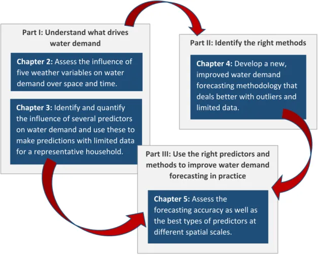
The main aims and objectives of this thesis and the way these are linked with each other are summarised in Figure 1.2. The first part of this work (Part I, Figure 1.2) is dedicated to understanding the drivers of water demand, as well as how these can be used to make predictions. The second part of the analysis focuses on developing a new, improved methodology that can address several of the main issues in water demand forecasting (e.g. lack of data, peak

consumption days) (Part II, Figure 1.2). Finally, the third part combines the knowledge acquired from parts I and II, to explore demand forecasting at different levels of spatial aggregation (Part III, Figure 1.2).

Figure 1.2 Overview of the thesis structure and the main topics that are addressed in

each chapter.

Part I: Understand what drives water demand

Chapter 2: Assess the influence of

five weather variables on water demand over space and time.

Chapter 3: Identify and quantify

the influence of several predictors on water demand and use these to make predictions with limited data for a representative household.

Part II: Identify the right methods

Chapter 4: Develop a new,

improved water demand forecasting methodology that deals better with outliers and limited data.

Part III: Use the right predictors and methods to improve water demand

forecasting in practice

Chapter 5: Assess the

forecasting accuracy as well as the best types of predictors at different spatial scales.

(33)

33

1.4.

Thesis overview

The thesis is divided into four methodological chapters (see chapters 2 - 5) and a conclusions chapter (see chapter 6), as well as three appendices (see

appendices A-B), containing supporting information for chapters 2, 4 and 5, respectively. Each one of the four methodological chapters corresponds to a research paper (for details see the following section) and addresses one of two aspects that are inherently connected to each other, understanding and

modelling water demand. A literature review as well as a description of the data that are used in this study, along with the cleaning and processing of this data are available as part of each chapter. A brief summary of the chapters and appendices is provided in the following:

Chapter 2 (addressing objective 1) focuses on identifying the influence of the weather over space and time. An extensive, big-data analysis is performed that disaggregates consumption into different household types, days and times of the day. The effect of five weather variables, air and soil temperature, humidity, sunshine duration and rainfall is examined for each segmentation of

consumption.

Chapter 3 (addressing objective 2) expands on this work by investigating the influence and predictive capability of several household, temporal and weather characteristics on water consumption using a machine learning approach. A Random Forest model is trained on daily consumption records using a variety of explanatory variables, in order to predict daily demand for a representative household. Three interpretable machine learning techniques are also used in order to investigate the influence of these predictors (household, temporal and weather characteristics) on the model’s output.

Chapter 4 (addressing objective 3) identifies the tools and methods that can enhance modelling accuracy, for different forecasting aims. As part of this effort, several machine learning models are compared for predictions of daily water consumption one day ahead. The model’s performance is assessed for all days in the data as well as peak days, i.e. the 10% of days with the highest

consumption. In addition, four bias correction methods are used in order to improve the problem of bias towards the mean, which is a very common, re-occurring problem in the literature that is often overlooked.

(34)

34

Chapter 5 (addressing objective 4) compares the prediction accuracy as well as the best types of variables (e.g. weather, temporal or household characteristics) at different levels of spatial aggregation. For this purpose, several Gradient Boosting Machines are trained on past consumption data, for different household group sizes (from 5 to 600 households) and compared for their accuracy in making predictions with one day lead time. Next, eight model configurations are trained and tested at three levels of spatial aggregation. Predictions are compared for one to seven days into the future, for all days in the data, as well as peak consumption days.

Chapter 6 provides an overview of the work performed, the key results and contributions of the study, as well as recommendations for further research. Appendix A. Provides supporting information for chapter 2.

Appendix B. Provides supporting information for chapter 5.

1.5.

Published work and other resources

The data used in this study is not publicly available and can be requested from different sources. The water consumption and household characteristic data was made available by Wessex Water (www.wessexwater.co.uk) and is

protected under a non-disclosure agreement. Interested parties can ask for data access directly from Wessex Water. The weather data was collected and

became available by the Meteorological Office of the UK (Met Office) (https://www.metoffice.gov.uk). This data was provided to the author for research purposes only and is available for purchase or under request by the Met Office.

All code for the analysis was developed by the author in R (unless explicitly stated within the thesis) and is available at the following github repository: https://github.com/mariaxen/DemandForecasting.

The work that was carried out during this PhD is summarised in four journal papers that have been published or are currently under review (see chapters 2-5). Part of the work that was carried out during this PhD project is also

presented in three conference papers that are available online and are not part of this thesis. A list of all journal and conference publications that were

(35)

35

1.5.1.

PhD candidate’s publications

Journal Papers

Xenochristou, M., Kapelan, Z., and Hutton, C. (2019). Using smart demand-metering data and customer characteristics to investigate the influence of weather on water consumption in the UK. J. Water Resources Planning and Management, doi: 10.1061/(ASCE)WR.1943-5452.0001148.

Xenochristou, M., Hutton, C., Hofman, J., and Kapelan, Z. (2019). A new approach to forecasting household water consumption. J. Water Resources Planning and Management (under review).

Xenochristou, M., and Kapelan, Z. (2019). An ensemble stacked model with bias correction for improved water demand forecasting. Urban Water Journal (under review).

Xenochristou, M., Hutton, C., Hofman, J., and Kapelan, Z. (2019). Water demand forecasting accuracy and influencing factors at different spatial scales using a Gradient Boosting Machine. Water Resources Research (under review). Conference Papers

Xenochristou, M., Kapelan, Z., Hutton, C., and Hofman, J. (2017): CCWi2017: F42 Identifying relationships between weather variables and domestic water consumption using smart metering. Available from:

https://figshare.shef.ac.uk/articles/CCWi2017_F42_Identifying_relationships_be tween_weather_variables_and_domestic_water_consumption_using_smart_me tering_/5364565/1.

Xenochristou, M., Kapelan, Z., and Hutton, C. (2018): HIC2018: Smart water demand forecasting: Learning from the data. Available from:

https://easychair.org/publications/open/qpH8.

Xenochristou, M., Blokker, M., Vertommen, I., Urbanus, J.F.X., and Kapelan, Z. (2018): CCWi2018: 032 Investigating the Influence of Weather on Water

Consumption: a Dutch Case Study. Available from:

(36)

36

2.1.

Introduction

Water availability is a major concern for water utilities in the UK (Water UK, 2016), because of a growing risk of severe drought impacts, due to changes in the climate and population growth. Accurate projections of demand are an essential part of their short-term forecasting, as well as long-term strategic planning. Managing household water use can lead to a reduction in the requirement for infrastructure investments, help secure water supply in the future, as well as save household energy use and greenhouse emissions (Bello-Dambatta et al., 2014). However, despite the clear benefits, few studies in the

This chapter was published as a Technical Paper in the Journal of Water Resources, Planning and Management (ISSN: 1943-5452). This publication has been slightly modified in order to improve consistency throughout the thesis. The chapter was written by Maria Xenochristou but has benefited from the comments of the co-authors, Zoran Kapelan and Chris Hutton.

Citation: Xenochristou, M., Kapelan, Z., and Hutton, C. (2019). Using smart

demand-metering data and customer characteristics to investigate the influence of weather on water consumption in the UK. J. Water Resources, Planning and

Management, 36, 3161-3174, doi: 10.1061/(ASCE)WR.1943-5452.0001148.

THE INFLUENCE OF WEATHER

ON WATER CONSUMPTION

(37)

37

literature have focused on water demand forecasting in the UK (Parker and Wilby, 2013).

The advent of smart meters in the late 1990s made water consumption data available at very high temporal (minutes or even seconds) and spatial (household) resolution, enabling a better understanding of the patterns of domestic water consumption (Agthe and Billings, 2002; Schleich and

Hillenbrand, 2008; Fox et al., 2009). Such data can be used to model demand at the household (or even micro-component) level and thus maintain the heterogeneity derived from the users’ unique characteristics and individual water uses (Parker and Wilby, 2013; Cominola et al., 2015). In addition to household, societal, economic and natural factors, the advance of smart metering allows to account for temporal variations in consumption.

The current chapter proposes a systematic, disaggregated methodology that utilises smart demand metering data in order to identify customer and temporal segments of consumption that are more sensitive to weather changes. It utilises simple statistical methods that could enable the development of improved water demand forecasting models and the implementation of effective demand

management strategies. As it can be seen from the next section, a systematic analysis of the weather influence on water consumption by using such data has not been conducted before.

2.2.

Water demand influencing variables

Many variables have been investigated in the water demand literature as drivers of water consumption. These can be divided into temporal and household

characteristics that are or can be known to water utilities, as well as weather fluctuations that are unpredictable in nature. Since the former follow a relatively stable or periodic behaviour, they are easier to account for and thus it is the influence of the weather that is of high interest to network operators.

2.2.1.

Temporal characteristics

Seasonal changes in water consumption, as well as weekly and daily patterns are a widely observed phenomenon (Agthe and Billings, 2002; Cole and

Stewart, 2013; Gurung et al., 2014; Parker, 2014; Romano and Kapelan, 2014). Typically, water demand reaches a peak during the summer months, when the

(38)

38

water is used for outdoor activities, such as filling water pools or gardening, as well as personal hygiene (Downing et al., 2003; Cole and Stewart, 2013). In a study by Parker (2014) with micro-component data from 100 households in the southeast of the UK, external use showed the highest difference between seasons, followed by shower use. In the same study (Parker, 2014), a weekly cycle was observed for certain water uses, suggesting increased water

consumption for washing machines over the weekend. On the other hand, Cole and Stewart (2013) found that water used for irrigation typically occurs between 2 am and 6 am, while water is used for showering between 7 am and 12 pm, as well as 5 pm and 9 pm.

2.2.2.

Household characteristics

According to several studies (Khatri and Vairavamoothry, 2009; Mamade et al., 2014; Parker, 2014), socio-demographic variables are the most important for daily consumption patterns. Consumers that live in higher-valued areas tend to have more water-using appliances and larger gardens, therefore an increased water-use (Linaweaver et al., 1967; Chang et al., 2010). This effect of income becomes even more relevant when water is used outdoors (Domene and Sauri, 2006).

In addition, the presence of garden and the property’s metering status have been found to influence the type of end-uses and the share among them, as well as the amount of water a household consumes. Among different household sizes and income groups, the presence of garden is one of the determining factors for increased water use (Domene and Sauri, 2006); households with larger lot sizes and no rainwater tanks tend to use more water for garden

irrigation (Loh and Coghlan, 2003). Water use for sprinkling and peak demands is more prominent among metered than unmetered customers (Hanke and Flack, 1968), whereas unmetered households’ external water use is also more responsive to meteorological variables (Parker, 2014).

2.2.3.

Weather characteristics

One of the major uncertainties relating to water consumption is the influence of the weather. A number of papers investigated the effect of weather on water demand (Miaou, 1990; Griffin and Chang, 1991; Agthe and Billings, 2002; Gato

(39)

39

et al., 2007; Haque et al., 2014; Bakker et al., 2014; Beal and Stewart, 2014; Dos Santos and Pereira, 2014).

Within a variety of weather variables, temperature and rainfall are the ones that are frequently suspected to have an influence on consumption. However, many others such as soil moisture, irradiation, sunshine hours and dry days also appear in the literature (Downing et al., 2003; Goodchild, 2003; Parker, 2014). Most studies found a strong relationship between air temperature and water consumption (Downing et al., 2003; Adamowski, 2008; Cole and Stewart, 2013; Willis et al., 2013; Beal and Stewart, 2014), whereas a much weaker one was identified for rainfall (Downing et al., 2003; Goodchild, 2003; Cole and Stewart, 2013; Beal and Stewart, 2014). Adamowski (2008) concluded that rainfall occurrence rather than amount correlates better with water consumption, whereas the occurrence/non-occurrence of rainfall, five days prior, is an even better predictor of daily water demand.

Several authors used linear models to quantify the effect of the weather on consumption (Jain et al., 2001; Downing et al., 2003; Goodchild, 2003; Khatri and Vairavamoothry, 2009; Browne et al., 2013; Parker, 2014). Parker (2014) concluded that all indoor micro-components are linearly related to maximum temperature, sunshine hours and amount of rainfall. A non-linear relationship was identified between temperature and external water use, creating the need to identify thresholds of sensitivity to weather variables and piecewise

regression techniques (Parker, 2014). Downing et al. (2013) concluded that most of the climate change impact on water use will be due to baths and showers. Parker (2014) on the other hand found that shower use is less sensitive to weather changes compared to external consumption, whereas washing machine use can also be weather dependent. More specifically, Parker (2014) concluded that an increase in temperature and sunshine hours can cause an increase in outdoor and shower use, whereas an increase in sunshine hours and decrease in rainfall can cause an increase in washing machine use.

2.2.4.

Summary

Household water use in the UK reflects a variety of time and space dependent variables (Parker and Wilby, 2013). Thus, taking a holistic view of climate effects, as well as temporal and behavioural drivers, is essential in order to

(40)

40

forecast demand (Parker, 2014). Although different temporal and social patterns in water use have been widely investigated, the connection between these and the weather has still not been made.

This study performs an in-depth analysis based on a unique water consumption dataset that is based on real and high frequency observations of water use (i.e. smart demand metering data), from a rather large number of houses located in the southwest of the UK. These consumption data are accompanied by equally detailed information on customer and property characteristics, providing a unique opportunity to explore how different days and water users are influenced by weather changes. Further details about the data used in this study can be found in the next section.

2.3.

Data

The current study is based in the UK, more specifically in the southwest of England (Dorset, Somerset, Wiltshire and Hampshire). It utilises an extensive dataset that comprises of:

 Smart demand metering data collected from 1,793 properties for a three year period (10/2014 - 09/2017) at 15-30 minute intervals;

 Property characteristics, including garden sizes, rateable values and metering statuses;

 Customer characteristics, comprised of acorn groups and types as well as occupancy rates. Acorn is a geodemographic segmentation of the UK’s population based on social factors and population behaviour and it is used to provide an understanding of the different types of customers (CACI, 2014);

 Weather data collected at hourly to daily intervals for the analysed time-period (10/2014 - 09/2017). The weather data was collected from hundreds of stations across the Southwest and acquired as part of the Met Office Integrated Data Archive System (MIDAS) Land and Marine Surface Stations Data (Table 2.1) (Met Office, 2006a; Met Office, 2006b; Met Office, 2006c; Met Office, 2006d; Met Office, 2006e). However, only 56 of them are included in the analysis, based on their proximity to the properties in the dataset.

(41)

41

Since the properties in the dataset are scattered over a relatively large area, daily and hourly information from multiple weather stations is used to calculate one daily value for each weather variable. In order to do this, a weight is

assigned to each station, based on the amount of properties that are the closest to it, as opposed to all other weather stations in the area.

The climate in England is characterised by mild temperatures and rainfall well-distributed all year round. Specifically, maximum air temperature averaged from 1981 to 2010 varied from 6.9°C to 20.9°C and sunshine duration from 54.2 to 193.5 hours in total from January to July, respectively (Met Office, 2012). Monthly rainfall varied between 58.4mm and 91.7mm, for May and October, respectively, whereas according to Met Office statistics from 1981 to 2010, it rains on average 132.8 days in a year (Met Office, 2012).

The weather over the analysed time period (10/2014 - 09/2017) in the south and southwest of England was fairly average, with the exception of some ho