LQR/PID Controller Design of PLC-based Inverted Pendulum

LQR/PID Controller Design of PLC-based

Inverted Pendulum

Kaset Sirisantisamrid, Napasool Wongvanich

∗

, Suphan Gulpanich, and Narin Tammarugwattana

Abstract—This paper presents an LQR based PID controller to control the inverted pendulum system. The control design employs a control zoning approach whereby the entire pendu-lum system is divided into two regions: a normal pendupendu-lum region and the inverted pendulum region where the system is approximately linear close to the upright position. The LQR architecture is used to obtain optimal gains for the PID controller. An algebraic approach is also presented for selection of Q and R matrices. Experimental implementations with a PLC based system show that the computed gains yield the most stable controlled responses compared to the gains chosen through trial and errors.

Index Terms—LQR control, PID control, PLC, Inverted Pendulum

I. INTRODUCTION

T

HE classical Proportional Integral Derivative (PID) controller has remained the most popular industrial controller over the last six decades, despite the enormous hosts of development over the same period [1]. Various PID tuning methods have been developed by a number of re-searchers in the last 40 years. Developments in evolutionary algorithms and particle swarm optimization have led to the application of these methods for PID tuning [2], [3]. Other PID tuning approaches include the direct search algorithms and online optimization based approaches [4], [5]. Although these methods have resulted in the automatic tuning of the PID controllers, they require significant computational loading, and are not suitable for real time applications.

The Inverted Pendulum system is an inherently unstable system which is coupled with highly nonlinear dynamics. This feature alone makes the inverted pendulum system a challenging one, and also making it a primitive benchmark for comparing the various control approaches. Several ad-vanced control designs have been presented, including fuzzy logics [6], [7]. These approaches however, require large training sets, and for the case of fuzzy based designs, a large set of rules which further complicates the control for higher order systems.

The Linear Quadratic Regulator (LQR) is well known in modern control, and besides the PID has been widely used. The LQR is used to obtain maximal performance of the system by minimizing the cost function relating the states and the control input. Through the use of optimal control theory, LQR is reduced to the solving of Algebraic Riccati Equation (ARE) to obtain the transformation matrixP. The

Manuscript received December 05, 2017; revised January 23, 2018 Kaset Sirisantisamrid, Napasool Wongvanich, Suphan Gulpanich and Narin Tammarugwattana are with the Department of Instrumentation and Control Engineering, Faculty of Engineering, King Mongkut’s Institute of Technology Ladkrabang, Bangkok, Thailand. E-mail: ([email protected],[email protected],[email protected], [email protected]).

∗_{Corresponding author}

weight matricesQandRare usually obtained through trial-and-error and thus sub-optimal. Bryson [8] developed the iterative tuning algorithm for selectingQandR. Kumar [9] developed an algebraic method of selecting the Q and R

matrices for a3×3system. This work extends this method to a5×5system for the application of controlling the nonlinear inverted pendulum system. Furthermore, to ensure simplicity of the controller designs, a control-zoning approach is also employed.

II. METHODOLOGY

A. The LQR controller outline

Consider the following linear-time invariant system de-scribed in the state-space form defined:

˙

x=Ax+bu (1a)

y=Cx (1b)

x≡[x1, x2, . . . , xn]T,x0≡

x10, . . . , xn0

T

(1c)

where xi = xi(t), i=1,...,n is a quantity of state i at time

t (s), x is the n×1 state vector, x0 is the initial state vector, y is the measurement state vector, u is the input. The main assumption here is that the input u is time-dependent only, and does not depend onx0. The conventional Linear Quadratic Regulator (LQR) control seeks an optimal controlleruoptthat minimizes the cost function:

J =

Z ∞

0

xTQx+uTRudt (2)

whereQ=QT is a positive semidefinite matrix, and Ris a positive definite matrix. MatrixQis the matrix penalizing the deviation of the states from the equilibrium, while matrix

Ris the matrix penalizing the control input size.

Through the use of optimal control theory, the optimal gain vectorK is given by:

K=R−1BTP (3)

where matrixP(n×n)is the solution of the algebraic Riccati Equation defined:

B. Algebraic method for selecting theQand Rmatrices

Consider a specific fifth order state space system with the following state matrices:

A=      

0 1 0 0 0

0 a22 0 a24 0

0 0 0 1 0

0 0 0 0 1

0 a52 0 a54 0

     

,B=

0, b2,0,0, b5

T

(5a)

C=c1, . . . , c5

(5b)

This state space representation is typical for optimal tuning designs of PID controllers using the LQR theory. The pro-cedure of LQR controller design requires the minimization of the cost function J of Equation (2). The state feedback control law that minimizesJ is:

u=−Kx (6)

where the optimal gain vector Kis given by Equation (3). Suppose that the weight matricesQandR, as well as the transformation matrix Pare chosen as defined:

Q=       q1 q2 q3 q4 q5      

,P= 

  

p11 p12 . . . p15 p21 p22 . . . p25 . . . . p51 p52 . . . p55



  

(7)

R=r (8)

where r is an arbitrarily chosen scalar. Consider now the closed loop state equation defined:

˙

xc= (A−BK)xc (9)

wherexcis the closed loop state. For stability the eigenvalues

of the closed loop state transition matrixA−BKshould all be negative, in other words, all lie on the left hand plane in a pole-zero diagram. The characteristic equation of the closed loop state transition matrix is:

f(s) =p1s+p2s2+p3s3+p4s4+s5= 0 (10)

where:

p1= a22b2b5p23+a22b

2

5p35−a24b2b5p12−a24b25p15

r

−a52b22p23−a52b2b5p35+a54b22p12+a54b2b5p15

r (11a)

p2= −

a22b2b5p24−a22b25p45+a24b2b5p22+a24b25p25+a52b22p24

r a52b2b5p45−a54b22p22−a54b2b5p25

r

+a22a54r−a24a52r+b2b5p23+b25p35

r (11b)

p3=−a22b2b5p25−a22b

2

5p55−b22a52p25−a52b2b5p55−b22p12

r

−b2b5p15−b2b5p24−b25p45+a54r

r (11c)

p4=−−

b2

2p22−2b2b5p25−b25p55+a22r

r (11d)

The desired characteristics of the fifth order system, for a givenξandωn, can be written:

fdesired(s) =s(s+ξωn)2(s2+ 2ξωn+ωn)2

=s5+ 4ξωns4+ω2n(5ξ

2_{+ 1)s}3

+ 2ω_n3ξ(ξ2+ 1)s2+ω_n4ξ2s (12)

Equating the co-efficients of Equation (12) to Equations (11a) - (11d), and assuming thatp12,p13,p15,p24,p25,p45 andp55are known, yields a system of three equations in three unknowns, which is solved in Maple to yield the values for p22,p23 andp35:

p22=_b2 1 2(−a22b5+a52b2)

(−a22p55+ 2p45)b35

+ 2(1

2p55a52+p24+p15)b2b 2 5+ (2b

2 2p12 −10r(₁₀1a2₂₂+2₅ωnξa22 + (ξ2+1₅)ωn2+

1 5a54))b5

+ 4a52r(ξωn+1₄a22)b2

(13a)

p23=_b2 1 2(−a22b5+a52b2)

−a24b45p45−(p45a222−p35a22

+ (p15+p24)a24−p45a54)b2b35+ ((−p24a222

+ 2p45a52a22−p12a24−p35a52+a54(p15

+p24))b22+ 5a24r((ξ2+1₅)ω2+4₅ωξa22

+1₅a2₂₂+1₅a54))b25−(2((−p24a22a52+1₂p45a252 −1

2a54p12)b 2

2+ (ξa22(ξ2+ 1)ω3+a54(5₂ξ2+1₂)ω2

+ 2ξ(a22a54+a24a52)ω+a22a24a52+1₂a254)r))b2b5

+ 2(−1 2p24b

2

2a52+ ((ξ3+ξ)ω3+ 2ωξa54

+1₂a24a52)r)a52b22

(13b)

p35=_b2 1 2(−a22b5+a52b2)

−b22p12−b5(a52p55

+p15+p24)b2+ (a22p55−p45)b25+ 5r((ξ2

+1₅)ω2+1₅a54)

(13c)

Consider now the element-wise form of the algebraic Riccati Equation:      

0 0 0 0 0

1 a22 0 0 a52

0 0 0 0 0

0 a24 1 0 a54

0 0 0 1 0

         

p11 p12 . . . p15 p21 p22 . . . p25 . . . . p51 p52 . . . p55

    +    

p11 p12 . . . p15 p21 p22 . . . p25 . . . . p51 p52 . . . p55

         

0 1 0 0 0

0 a22 0 a24 0

0 0 0 1 0

0 0 0 0 1

0 a52 0 a54 0

      +       q1 q2 q3 q4 q5       −1 r    

p11 p12 . . . p15 p21 p22 . . . p25 . . . . p51 p52 . . . p55



  

×

0, b2,0,0, b5

T

0, b2,0,0, b5

×    

p11 p12 . . . p15 p21 p22 . . . p25 . . . . p51 p52 . . . p55



  

=0 (14)

is readily solved for the elements q1, . . . , q5 in Maple:

q1=

b2p12+b5p215

r (15a)

q2=

1

r(−2a22p22−2a52p25−2p12)r

+ (b2p22+b5p25)2 (15b)

q3=

b2p23+b5p235

r (15c)

q4= (−2

a24p24−2a54p45−2p34)r+(b2p24+b5p45)2)

r (15d)

q5= b2

2p225+ 2b2b5p25p55+b25p255−2p45r)

r (15e)

The optimal gainKoptof Equation (3), in element wise form,

is now:

K=

b2p12+b5p15

r ,

b2p22+b5p25

r ,

b2p23+b5p35

r , b2p24+b5p45

r ,

b2p25+b5p55

r

T

(16)

where the elements are computed by substituting Equations (13a) - (13c) into Equation (16).

III. RESULTS ANDDISCUSSION

A. The Inverted Pendulum system setup

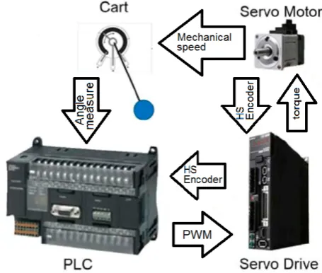
[image:3.595.314.542.56.249.2] [image:3.595.62.293.70.203.2]

The setup of the inverted pendulum on a cart is shown in Figure 1. The cart can move back and forth along a support rail. The cart also has two wires, one is connected to the servo driver (R88D-KP01H), which is in turn connected to a PLC of Sysmac C-series CP1H 40 I/O model. The other wire is connected to the encoder which is for feedback of the cart position and velocity. The PLC sends out high frequency pulse signals to command the position controller of servo to achieve the required cart position and velocity. The system is connected to CX programmer for access and changing the controller gains via the PID(190) command of the PLC. A PLC datalogging system is also used for data acquisition and for viewing the control signals. Figure 2 shows the interaction between the PLC and the servo motors. All data are saved in a.txtfile, and can be viewed in MATLAB.

Fig. 1. The inverted pendulum on a cart

B. The Inverted Pendulum Model

Consider an inverted pendulum suspended on a moving cart as shown in Figure 3:

[image:3.595.309.544.298.386.2]

Fig. 2. The interaction between the PLC and the servo motors for the inverted pendulum system

Fig. 3. The inverted pendulum on a cart

The differential equations governing the motion of the inverted pendulum are defined:

(M+m)¨x+γ2x˙ =Fv+mlsinθ( ˙θ)2−mlcosθθ¨ (17a)

(I+ml2) ¨θ=mglsinθ−mglcosθx¨ (17b)

whereM andmare the masses of the cart and pendulum re-spectively (kg),lthe pendulum length (m),gthe gravitational constant (m s−2),β1the damping constant of the cart (kg m s−1),Fv the applied force onto the cart,xthe cart position

andθthe pendulum angle. Equations (17a) and (17b) can be linearized to yield the following differential equations:

¨

x=−mg M θ−

γ2 Mx˙+

γ1

MV (18)

¨

θ= (M +m)g

ml θ− γ2 M lx˙−

γ1

M lV (19) Equations (18) and (19) can be expressed as state space equations where the state matrices are:

A= 

  

0 0 1 0

0 0 0 1

0 −mg_M −γ2

M 0

0 (M+_mlm)g −γ2

M l 0



  

, B= 

  

0 0

γ1

M

−γ1

M l



  

(20)

C. The Inverted Pendulum Control: Defining the control regions

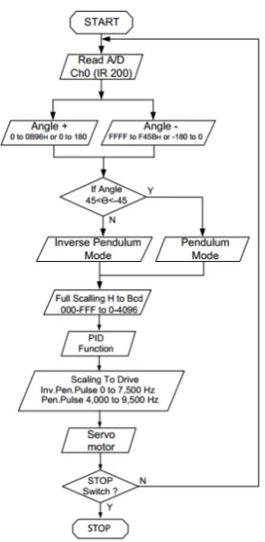
[image:3.595.52.289.533.649.2]

[image:4.595.100.243.251.391.2]

and thus designing a controller on the linearized dynamical model itself would likely result in a sub-optimal design. To achieve optimal design the entire system is thus divided into two regions in which the reference angle θ=0 is taken from the upright position: the normal pendulum region and the inverted pendulum region, where the normal pendulum region is between -45◦≤θ≤45◦and the inverted pendulum region is between 45◦ < θ < -45◦ as shown in Figure 4. This division is similar to the control zoning approaches used in many industrial PLCs in level and temperature controls. For future references the inverted pendulum region will also be termed the linear region. Figure 5 shows the flowchart describing the implementation of the inverted pendulum control through a PLC. It is seen that the pendulum regions defined in Figure 4 is specified into the PLC system.

[image:4.595.311.548.384.509.2]

Fig. 4. Defining the pendulum regions withθ= 0◦as reference

Fig. 5. The PLC based inverted pendulum system flowchart

D. Controlling the inverted pendulum in the normal pendu-lum region

In controlling the inverted pendulum setup in the normal pendulum region, a simple PID controller is used to allow implementation onto the PLC. In this region the proportional gain Kp is set to be large while the integral time Ti is

set small, to allow maximum increase of the cart speed in order to generate sufficient forces to swing the pendulum. The minimal Ti value is set to allow minimal time for

the pendulum to reach the inverted pendulum region. For simplicity, the set of gains for the controller in this region is determined through trial and error of the simulated model in MATLAB, and is given by:

Kp= 1.0, Ti= 0.1, Td= 20 (21)

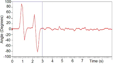
The implementation of the PID gains of Equation (21) onto the apparatus of Figure 1 is now done through the PLC commandPID(88). Figure 6 shows the responses from the PLC datalogger, where the set point (green) is fixed at 46◦to ensure that the pendulum now reaches the inverted pendulum region. The red signal denotes the control response of the pendulum. Datalogging begins att= 0.8 s, and ends when the system finally reaches the inverted pendulum region at t= 4.7 s. This means that the system achieves the inverted pendulum region int= 3.9s.

Fig. 6. The control responses from implementing Equation (21) onto the apparatus of Figure 1.

E. Controlling the inverted pendulum in the inverted region

As discussed in Section III-C, the inverted pendulum region is one where linear model approximations can be sufficiently made to the dynamics of the pendulum. In this light, designing a simple PID controller whose gains are optimally tuned can be done in conjunction with another controller architecture such as LQR. Since PID controllers concerns with the errore(t), such function and their associ-ated derivativese˙and¨ehave to be defined as states to enable the use of LQR. In this respect, denote the position error as ex, the angular error eθ, where the relationships between

these errors and their desired set point valuesxd andθd are

defined:

ex=xd−x (22)

[image:4.595.102.249.442.742.2]

Substituting Equations (22) and (23) into the linearized differential Equations (18) and (19) and simplifying yields:

¨

ex=−a1eθ−a2e˙x−a3V (24)

¨

eθ=a4eθ−a5e˙x+a6V (25) where:

a1=− mg

M , a2= γ2

M, a3= γ1

M (26a)

a4=

(M +m)g

ml , a5= γ2

M l, a6= γ1

M l (26b)

[image:5.595.48.292.87.186.2]

where the physical parameters are given in Table I.

TABLE I

THE PHYSICAL PARAMETERS OF THE INVERTED PENDULUM SYSTEM.

Physical Description Pendulum Cart Support

Length 250 mm 300 mm 500 mm

Mass 156 g 450 g –

The statesx1 tox5 for this system are now defined:

x1=ex, x2= ˙ex, x3=

Z t

0

eθdt (27)

x4=eθ, x5= ˙eθ. (28)

The absence of the term Rt

0exdt is due to the fact that the control is primarily concerned with stabilization of the inverted pendulum at the upright position without regard to its position errors. Equations (24) and (25) can therefore be written as a state space system with the following state matrices:

Aθ=



    

0 1 0 0 0

0 −a2 0 a1 0

0 0 0 1 0

0 0 0 0 1

0 −a5 0 a4 0



    

, Bθ=0,−a3,0,0, a6

T

(29)

Although the inverted pendulum region was defined to lie within the angles of 45◦ < θ <-45◦, as depicted in Figure 4, some nonlinearities may still exist around the edge of the region, particularly during the transition from the normal pendulum region to the inverted pendulum region. In order to keep the controller design simple whilst coping with these nonlinearities, the overshoot is allowed to be quite large (≈ 90%). The settling time is designed to be 3 s. The damping factorζ and natural frequencyωn are related to the settling

timeTsand the percentage overshoot %OS by [10]:

ζ=_q −ln(%OS/100)

π2_{+ ln}2_(%OS/100)

(30)

ωn =

−ln(0.02p1−ζ2 ζTs

. (31)

Substituting %OS = 90 andTs= 3 into Equations (30) and

(31) yields:

ζ= 0.5 ωn= 4 (32)

To compute the LQR gains using the algebraic method of Section 2.2, first the parameterr is arbitrarily chosen to be

r= 0.1. The parametersp12,p13,p15,p24,p25,p45 andp55 are then chosen as follows:

p12= 0.2, p13= 0.25, p15= 0.25,

p24= 0.25, p45= 0.3p55= 0.25 (33)

Substituting the parameters of Equations (32) and (33), along with the parameters in Table I, into Equations (13a) - (13c), (15a) - (15e) and (16) yields:

Kdesign =

1,1,1,3,6T (34) The last three elements of matrix K are the proportional gain Kp, the integral gain KI and the derivative gain KD

of the conventional PID controller. The PLC version of the PID controller, however, slightly modifies the conventional PID controller whereKi andKd are defined in terms of the

integral timeTi and derivative timeTd [11]:

Ki=

Kp

Ti

, Kd=KpTd (35)

The set of gains in vector Kdesign is first simulated via the lqrcommand in MATLAB. Figure 7 plots the simulatedeθ

response. It is evident here that the maximum overshoot of eθat 90% occurs around 0.5 s, then reaches the steady state

[image:5.595.324.526.358.519.2]

at around 3.0 s as designed.

Fig. 7. The simulated control response withKdesignof Equation (34)

VectorKdesignin its present form is suitable only for

simu-lation on a computer aided design software such as MATLAB or Simulink. In order to implement the gains of Equation (34) on to the inverted pendulum apparatus of Figure 1, the last three elements of Kdesign need to be converted to the

PLC version of the PID controller. Substituting the last three element of vectorKdesign into Equation (35) and solving for

the integral timeTi and derivative timeTd yields:

Kp= 3, Ti= 1, Td = 2 (36)

The gains of Equation (36) is now implemented onto the in-verted pendulum apparatus of Figure 1 through the command

PID(88)as was done for the pendulum region. Figure??

[image:6.595.63.286.166.293.2]

reaches 0◦at around 3 s as designed. This was also expected since the controller designs already allowed the overshoot to be up to 90% to cater for the nonlinearity effects. These results show that having an allowable margin of errors could prove to be a useful approach in controller designs when there exists some unmodelled effects. This concept is already prevalent in many other engineering disciplines such as civil engineering.

Fig. 8. The angle error responses from implementing the controller of Equation (36) onto the apparatus of Figure 1.

To further test the set of gains of Equation (36) on the inverted pendulum apparatus, four other sets of gains are set as a comparison:

G1={Kp= 1, Ti= 1, Td= 1} (37a)

G2={Kp= 1, Ti= 1, Td= 2} (37b)

G3={Kp= 1, Ti= 2, Td= 1} (37c)

G4={Kp= 2, Ti= 1, Td= 2} (37d)

[image:6.595.51.289.629.685.2]

Each set of gains of Equations (36), (37a) - (37d) are implemented onto the inverted pendulum apparatus 8 times. For each of the trials, three possible scores based on the experimental stability of the controlled responses is noted. The trial is denoted “S” if the pendulum stays on the upright position without any vibration, in other words, the system is stable; “MS” if the pendulum vibrates while at the upright position, or in other words, being marginally stable, and “US” if the pendulum system is completely unstable, that is, does not stay on the upright position at all. Table II shows the experimental stability results.

TABLE II

THE EXPERIMENTAL STABILITY RESULTS OF THEPLC-BASED INVERTED PENDULUM DESIGNS FOR THE SET OF GAINS OFEQUATIONS

(36), (37A) - (37D).

Gains/Trial 1 2 3 4 5 6 7 8

{1,1,1} S US S US S US US US

{1,1,2} S MS S S US US US S

{1,2,1} S US US US S US US S

{2,1,2} US S US S S US MS S

{3,1,2} S S MS S S MS S S

It is seen from Table I that the designed set of gains of {3,1,2} results in the most stable pendulum system with 100% of the controlled responses being either completely stable or marginally stable. This result validates that the designed set of gains is capable of handling the nonlinearities that were still prevalent around the edges of the inverted pendulum region.

IV. CONCLUSION

This work has presented an LQR based PID controller to control the inverted pendulum system. To facilitate an integration with a PLC, the control design uses a control zon-ing approach where the entire pendulum is divided into two regions: a normal pendulum regions where the nonlinearities are inherent, and the inverted pendulum region where the system is approximately linear close to the upright position. The errors in position and angle are denoted control states to enable the use of the LQR architecture to obtain the optimal gains for the PID controller. An algebraic approach was also presented to allow a systematic method for selection of the

Q and R matrices, which in turn yielded an optimal set of control gainsKdesign. Experimental implementations with

the PLC based system show that the computed gains yield the most stable controlled responses compared to the gains chosen through trial and errors, which would be the case with implementations onto the real world system.

There are many other controller designs in the literature for the inverted pendulum system. However these methods typically make very strong assumptions on the validity of the system model. Although these controller designs share the flexibility of being tunable online to compensate for modelling errors, they typically require large amount of computational efforts. The approach in this paper uses the control zoning to effectively set an allowable margin of errors in face of unmodelled effects. This approach alleviates the computational loadings and simplify implementations. In any practical system the simpler the controller design the less chance of coding errors and hardware failures.

REFERENCES

[1] C. Knospe, “PID control”,IEEE Control Systems Magazine, Vol. 26, pp. 30-31, 2006.

[2] D.H. Kim and J.H. Cho,“Intelligent tuning of PID controller with disturbance function using immune algorithm,” Proc. of the IEEE Annual Meeting Fuzzy Information Processing, pp. 286-291, 2004. [3] M. I. Solihinet al., “Optimal PID controller tuning of automatic gantry

crane using PSO algorithm”,Proc. of the 5th International Symposium on Mechatronics and its Applications, pp. 1-5, 2008.

[4] H. Paganagopoulos et al., “Optimal tuning of PID controllers for first order plus time delay models using dimensional analysis”. IEE Proceedings, Vol. 149, no.1, pp. 32-40, 2002.

[5] C. Hwang and C. Y. Hsiao, “Solution of a non-convex optimization arising in PI/PID control design,”Automatica, Vol. 38, no.11, pp. 1895-1904, 2002.

[6] G. Rayet al., “Stabilization of inverted pendulum via fuzzy control”.

Journal of the institution of engineers (India) Electrical Engineering, Vol. 88, pp. 58-62, 2007.

[7] Y. M. Liuet al., “Real-time controlling of inverted pendulum by fuzzy logic”. Proc. of IEEE International Conference on Automation and Logistics, pp. 1180-1183, 2009.

[8] A.E. Bryson Jr. and Y. C. Ho, “Applied Optimal Control”, USA. 1975. [9] E. V. Kumar, J. Jerome, and K. Srikanth, “Algebraic approach for selecting the weighting matrices of linear quadratic regulator”, Proc. of the International Conference on Green Computing Communication and Electrical Engineering, pp. 1-6, 2014.

[10] G. F. Franklin, J. Da Powell, A. Emani-Naeini,Feedback Control of Dynamic Systems, 7th Ed.Pearson, 2015